Fully dynamic and memory-adaptative spatial approximation trees

Fully Dynamic and Memory-Adaptative Spatial

Approximation Trees

Diego Arroyuelo

Gonzalo Navarro

Nora Reyes

1

Depto. de Inform´atica

Center for Web Research

Universidad Nacional de San Luis

Dept. of Computer Science

Ej´ercito de los Andes 950

University of Chile

San Luis, Argentina

Blanco Encalada 2120, Santiago, Chile

f

darroy,nreyes

@unsl.edu.ar

[email protected]

Abstract

Hybrid dynamic spatial approximation treesare recently proposed data structures for

search-ing in metric spaces, based on combinsearch-ing the concepts of spatial approximation and pivot based algorithms. These data structures are hybrid schemes, with the full features of dynamic spatial approximation trees and able of using the available memory to improve the query time. It has been shown that they compare favorably against alternative data structures in spaces of medium difficulty.

In this paper we complete and improve hybrid dynamic spatial approximation trees, by pre-senting a new search alternative, an algorithm to remove objects from the tree, and an improved way of managing the available memory. The result is a fully dynamic and optimized data structure for similarity searching in metric spaces.

Key Words: databases, data structures, algorithms, metric spaces.

1

Introduction

“Proximity” or “similarity” searching is the problem of looking for objects in a set close enough to a query. This has applications in a vast number of fields. The problem can be formalized with the

metric space model[2]: There is a universeUof objects, and a positive real-valued distance function

d : UU ! R

+

defined among them, which satisfies the metric properties: strict positiveness

(d(x;y) = 0 , x = y), symmetry(d(x;y) = d(y;x)), andtriangle inequality (d(x;z) 6 d(x;y)+

d(y;z)). The smaller the distance between two objects, the more “similar” they are. We have a finite

databaseS U that can be preprocessed to build an index. Later, given aqueryq 2 U, we must

retrieve all similar elements in the database. We are mainly interested in therange query: Retrieve all elements inS within distancertoq, that is,fx2S; d(x;q)6rg.

Generally, the distance is expensive to compute, so one usually defines the search complexity as the number of distance evaluations performed. Proximity search algorithms build an index of the database to speed up queries, avoiding the exhaustive search. Many of these indexes are based on pivots (Section 2).

In this paper we complete and improve a hybrid index for metric space searching built on the

dsa–tree [3], an index supporting insertions and deletions that is competitive in spaces of medium difficulty, but unable of taking advantage of the available memory. This was enriched with a pivoting scheme in [1]. Pivots use the available memory to improve query time, and in this way they can beat any other structure, but too many pivots are needed in difficult spaces. Our new structure was still dynamic and made better use of memory, beating bothdsa-treesand basic pivots. Now we present a new search alternative, a deletion algorithm, and a way of managing the available memory forhybrid dynamic spatial approximation trees. In this way we complete and improve our previous work [1].

2

Pivoting Algorithms

Essentially, pivoting algorithms choose some elementsp

i from the database

S, and precompute and

store all distancesd(a;p i

)for all a 2 S. At query time, they compute distancesd(q;p i

)against the

pivots. Then thedistance by pivotsbetweena 2Sandqgets defined asD(a;q)=max p

i

jd(a;p i

)

d(q;p i

)j.

It can be seen that D(a;q) 6 d(a;q) for all a 2 S; q 2 U. This is used to avoid distance

evaluations. Eacha such thatD(a;q) >r can be discarded because we deduced(a;q) >r without

actually computingd(a;q). All the elements that cannot be discarded this way are directly compared

againstq.

Usually pivoting schemes perform better as more pivots are used, this way beating any other index. They are, however, better suited to “easy” metric spaces [2]. In hard spaces they need too many pivots to beat other algorithms.

3

Dynamic Spatial Approximation Trees

3.1

Insertion Algorithm

Thedsa–treeis built incrementally, via insertions. The tree has a maximum arity. Each tree nodea

stores a timestamp of its insertion time,time(a), and its covering radius,R (a), which is the maximum

distance to any element in its subtree. Its set of children is calledN(a), theneighborsofa. To insert

a new elementx, its point of insertion is sought starting at the tree root and moving to the neighbor

closest tox, updatingR (a)in the way. We finally insertxas a new (leaf) child ofaif (1)xis closer

toathan to anyb 2N(a), and (2) the arity ofa,jN(a)j, is not already maximal. Neighbors are stored

left to right in increasing timestamp order. Note that the parent is always older than its children.

3.2

Range Search Algorithm

The idea is to replicate the insertion process of elements to retrieve. That is, we act as if we wanted to insertqbut keep in mind that relevant elements may be at distance up torfromq, so in each decision

for simulating the insertion ofqwe permit a tolerance ofr. So it may be that relevant elements were

inserted in different children of the current node, and backtracking is necessary.

Note that, at the time an element x was inserted, a node a may not have been chosen as its

parent because its arity was already maximal. So, at query time, we must choose the minimum distance to x only among N(a). Note also that, when xwas inserted, elements with higher

times-tamp were not yet present in the tree, so x could choose its closest neighbor only among older

elements. Hence, we consider the neighbors fb 1

;:::;b k

g of a from oldest to newest,

disregard-ing a, and perform the minimization as we traverse the list. That is, we enter into subtree b i if d(q;b

i

)6min(d(q;b 1

);:::;d(q;b i 1

))+2r.

We use timestamps to reduce the work inside older neighbors. Say thatd(q;b i

)>d(q;b i+j

)+2r.

We have to enter subtreeb

i anyway because b

i is older. However, only the elements with timestamp

smaller thantime(b i+j

)should be considered when searching insideb

i; younger elements have seen b

i+j and they cannot be interesting for the search if they are inside b

i. As parent nodes are older than

their descendants, as soon as we find a node inside subtreeb

i with timestamp larger than

time(b i+j

)

we can stop the search in that branch.

Algorithm 1 performs range searching. Note that, except in the first invocation,d(a;q)is already

known from the invoking process.

3.3

Deletion Algorithm

To delete an elementx, the first step is to find it in the tree. In which follows, we do not consider the

location of the object as part of the deletion problem, although in [3] we have shown how to proceed if necessary. It should be clear that a tree leaf can always be removed without any complication, so we focus on how to remove internal tree nodes.

The deletion of elements by rebuilding subtreesensures that the resulting tree is exactly as if the deleted element had never been inserted. Thus, no degradation can occur due to repeated deletions. In such algorithm, when nodex2N(a)is deleted, we disconnectxfrom the main tree. Hence all its

descendants must be reinserted. Moreover, elements in the subtree ofathat are younger thanxhave

been compared againstx to decide their insertion point. Therefore, these elements, in absence ofx,

RANGESEARCH(Nodea; Queryq; Radiusr; Timestampt)

1. if time(a)<t ^ d(a;q)6R (a)+r then

2. if d(a;q)6r thenreporta

3. d min

1

4. for b i

2N(a)in increasing timestamp order do

5. if d(b i

;q)6d min

+2r then

6. k minfj>i; d(b i

;q)>d(b j

;q)+2rg

7. RANGESEARCH(b i

;q;r;time(b k

))

8. d

min

minfd min

; d(b i

;q)g

Algorithm 1: Range query algorithm on adsa–treewith roota.

thanx that descend froma (i.e. those whose timestamp is greater, which includes its descendants)

and reinsert them into the tree, leaving the tree as ifxhad never been inserted.

If we reinsert the elements younger thanxlike completely new elements, that is if they get fresh

timestamps, we must search the appropriate point of reinsertion beginning at tree root. On the other hand, if we maintain their timestamp we can start the reinsertion process from a, so we can save

many comparisons. In order to leave the resulting tree exactly as ifx never had been inserted, we

must reinsert the elements in the original order, that is, the elements must be reinserted in increasing order of timestamp.

Therefore, when node x 2 N(a) is deleted we retrieve all the elements younger thanx from the

subtree rooteda, then disconnect them from the main tree, sort them in increasing order of timestamp

and reinsert them one by one, searching their reinsertion point froma.

Note that in this method the covering radii can become overestimated, because they are never reduced due to a deleted element. If we delete an element x, every a 2 A(x) such thatx was the

farthest element in its subtree will possibly have itsR (a) overestimated. In spite of it, this problem

does not seem to affect much search performance since it does not significantly degrade over time (see [4] for more details).

4

Fully Dynamic Sa–trees with Pivots

Hybrid dynamic sa–treeswere defined in [1], although without handling deletions. We review some of their main features and then present a deletion algorithm.

Pivoting techniques can trade memory space for query time, but they perform well on easy spaces only. Adsa–tree, on the other hand, is suitable for searching spaces of medium difficulty. However, it uses a fixed amount of memory, being unable of taking advantage of additional memory to improve query time. The idea is to obtain a hybrid data structure that gets the best of both worlds, by enriching

dsa–treeswith pivots. The result is better than both building blocks.

siblings of its ancestors, and its own siblings inN(a). At query time, when we reach node x, some

distances betweenqand the aforementioned elements have also been computed. So, we can use (some

of) these elements as pivots to obtain better search performance, without introducing extra distance computations. Next we present different ways to choose the pivots of each node.

4.1

H–DSAT1: Using Ancestors as Pivots

A natural alternative is to regard the ancestors of each node as its pivots. Let A(x) be the set of

ancestors of x 2 S. We define P(x) = f(p i

; d(x;p i

)); p

i

2 A(x)g. This set is computed during

insertion ofx, by storing some of the distance evaluations computed in this process. We storeP(x)

at each nodexand use it to prune the search.

4.1.1 Insertion Algorithm

To insert an elementx, we set P(x) = ;and begin searching for the insertion point of x. For each

nodea we choose in our path, we add(a;d(x;a))to P(x). When the insertion point ofxis found,

P(x)contains the distances to the ancestors of x. Note that we do not perform any extra distance

evaluations to buildP(x). Thus, the construction cost of a H–DSAT1 isthe sameof adsa–tree.

4.1.2 Range Search Algorithm

For range searching, we modify thedsa-treealgorithm to use the setP(x)stored at each tree nodex.

We recall that, given a set of pivots, the distance by pivotsD(a;q)is a lower bound ford(a;q).

Consider again Algorithm 1. If at step 1 it holds thatD(a;q) >R (a)+r, then surelyd(a;q) >

R (a)+r, and hence we can stop the search at nodeawithout actually evaluatingd(a;q). An element a in S is said to befeasible for query q if D(a;q) 6 R (a)+r. That is, is feasible that a or some

element in its subtree lies within the search radius ofq.

At search time, D(a;q) can be computed without additional evaluations of d. Suppose that we

reach node p

k of the structure and want to decide if the search must follow into the subtree of

x 2

N(p k

). At this point, we have computed all distancesd(q;p i

); p i

2 A(x). IfA(x) = fp

1 ;:::;p

k g,

then these distances ared(q;p 1

);:::;d(q;p k

). As the setP(x) =f(p 1

;d(x;p 1

));:::;(p k

;d(x;p k

))g

is stored in the node of x, then the distances d(x;p i

) and d(q;p i

) needed to compute D(x;q) are

present, at no extra costs. The distancesd(q;p

i

)are stored in a stack as the search goes up and down the tree. The setsP(x)

are also stored in root-to-xorder, for example in a linear array, so that references to the pivots inP(x)

(first component of pairs) are unnecessary to correctly computeD, and we save space.

The covering radius feasible neighbors of node a (feasible neighbors), denoted F(a), are the

neighborsb2 N(a)such thatD(b;q)6R (b)+r. The other neighbors are said to beinfeasibles.

At search time, if we reach nodea, only the feasible neighbors ofacould be taken into account, as

other subtrees can be discarded completely. Observe that these subtrees have been discarded usingD

and notdand, as we have explained,Dis computed for free. However, it does not immediately follow

that we obtain for sure an improvement in search performance. The reason is that infeasible nodes still serve to reduced

min in Algorithm 1, which in turn may save us entering into younger siblings.

RANGESEARCHH–DSAT1 (Nodea; Queryq; Radiusr;Timestampt)

1. if time(a)<t ^ d(a;q)6R (a)+r then

2. if d(a;q)6r thenreporta

3. d min

1

4. F(a) fb2N(a); D(b;q)6R (b)+rg

5. for b i

2N(a)in increasing timestamp order do

6. if b i

2F(a) ^ D(b

i

;q)6d min

+2rthen

7. if d(b i

;q)6d min

+2r then

8. k minfj>i; d(b i

;q)>d(b j

;q)+2rg

9. RANGESEARCHH–DSAT1(b i

;q;r;time(b k

))

10. ifd(b i

;q)has already been computedthend min minfd min ; d(b i ;q)g

Algorithm 2:Range searching for queryqwith radiusrin a H–DSAT1 with roota.

Now we present a new search alternative not devised in [1]. The idea is to use Dalong with the

hyperplane criterionto save distance computations at search time. For any feasible elementb i such

thatD(b i

;q) > d min

+2r, it holds thatd(b i

;q) > d min

+2r. Hence, we can stop the search in the

feasible nodeb

i without evaluating d(b

i ;q).

In which follows we present different alternatives of the search algorithm. The Algorithm 2 shows the first alternative.

However, in step 8 we run into the risk of comparing infeasible elements againstq. This is done

in order to use timestamp information as much as possible, but it introduces the undesired effect of reducing the benefits of pivots in our data structure. We present some improvements to this weakness.

Optimizing using D. We make use of D at search time not only to determine the feasibility of

a node and prune the search space saving distance evaluations, but also to decrease the number of infeasible elements that are compared directly againstqin step 8 of the algorithm. We search inside

b

i using the timestamp

tof a younger siblingb kof

b

i. Fortunately, some of the necessary comparisons

can be saved by making use of D. The key observation is that d(b i

;q) 6 D(b

j

;q)+2r implies d(b

i

;q) 6 d(b j

;q)+2r, so ifd(b i

;q) 6 D(b

j

;q)+2r we can conclude that b

j is not of interest in

step 8, hence saving the computation ofd(b j

;q). Although we save some distance computations and

obtain the same result, still there will be infeasible elements compared againstq. We call H–DSAT1D

this search method.

Using Timestamps of Feasible Neighbors. The use of timestamps is not essential for the correct-ness of the algorithms. Any larger value would do, although the optimal choice is to use the smallest correct timestamp. Another alternative is to compute a safe approximation to the correct timestamp, but ensuring that no infeasible elements are ever compared againstq. Note that every feasible neighbor

of a node will be compared againstqinevitably. If forb i

2F(a)it holds thatd(b i

;q)6d min

+2r, then

we compute the oldest timestamptamong the reduced setfb i+j

2F(a); d(b

i

;q)>d(b i+j

;q)+2rg,

and stop the search insideb

iat nodes whose timestamp is newer than

elements are compared againstq, and under that condition it uses as much timestamping information

as possible. We call H–DSAT1F this alternative.

4.1.3 Deletion Algorithm

We adapt the algorithm ofrebuilding subtrees[4] to delete an element x2 N(a)from the tree, such

that it takes into account the existence of pivots. The reinsertion process involve distance evaluations, some of which are already precomputed as pivot information. We show how to take advantage of this. Note thatais a pivot of every element in its subtree. In other words, the distanced(b;a)has been

stored inP(b), for everybin the subtree ofa. As a result, we can save at least one distance evaluation

for each element to be reinserted. Furthermore, ifyis an older sibling ofx, andyis a pivot (ancestor)

ofbthen we can save the distance evaluationd(b;y)when reinsertingb.

AsP(b)is stored using a linear array, the position ofd(b;a)inP(b)can be easily computed. Ifa

lies at leveliof the tree, thend(b;a)is at positioniof the array.

It is important to note that, after reinsertingb, the nodeaand the ancestors ofawill be ancestors

ofb. Then, we must keep inP(b)the distances betweenband the ancestors ofa. The other distances

inP(b)are discarded before reinsertingb. Finally, the new setP(b)is completed using some of the

distance evaluations produced at reinsertion time.

The deletion process ofx2N(a)can be resumed as follows. We retrieve all the elements younger

thanxfrom the subtree rooteda, then disconnect them from the main tree, discard the distances to the

pivots that are not of interest after reinserting the node, sort the nodes in increasing order of timestamp and reinsert them one by one (reusing some distances inP), searching their reinsertion point froma.

The result is very important: we do not introduce extra distance evaluations in the deletion process, and even more, the deletion cost can be reduced by using pivots.

4.2

H–D

2: Using Ancestors and their Older Siblings as Pivots

We aim at using even more pivots than H–DSAT1, to improve even more the search performance. At search time, when we reach a nodea, qhas been compared against all the ancestors and some of the

older siblings of ancestors ofa. Hence, we use this extended set of pivots for each nodea.

4.2.1 Insertion Algorithm

The only difference in a H–DSAT2 is in the P(x) sets we compute. Let x 2 S and A(x) =

fp 1

;:::;p k

gbe the set of its ancestors, wherep

i is the ancestor at tree level

i. Note thatp i+1

2N(p

i ).

Hence,(b;d(x;b))2P(x)if and only if (1)b 2A(x), or (2)p i

;p i+1

2A(x)^b 2N(p

i

)^time(b)<

time(p i+1

).

4.2.2 Range Search Algorithm

For range searching, to computeD(x;q)we need the distances betweenqand the pivots ofxstored

in a stack. But it is possible that some of the pivots of xhave not been compared againstq because

they were infeasible. In order to retain the same pivot order ofP(x), we push invalid elements into

the stack when infeasible neighbors are found. Dis then computed having this in mind. We define

the same variants of the search algorithm for H–DSAT2, which only differ from H–DSAT1 in the way

4.2.3 Deletion Algorithm

Now suppose we want to delete an element x 2 N(a) in H–DSAT2. Again, a is a pivot of each

elementbin the subtree rooteda. Thus, we can avoid at least one distance evaluation for element to

be reinserted. But we can do more. The comparisond(b;y)can be avoided, for ally 2 N(a) older

thanx, since those distances have been stored inP(b). The process of computing the position of the

distances inP(b) is not so direct as before: these must be computed as we retrieve the nodes to be

reinserted. Because of the features of H–DSAT2, it is possible that the deletion cost can be reduced even more.

5

Limiting the Use of Storage

In practice, available memory is bounded. Our data structures, as have been defined, use memory in a non-controlled way (each node uses as much pivots as the definition requires). This fact rules out our solutions for many real-life situations. We show how to adapt the structures to fit the available memory. The idea is to restrict the number of pivots stored in each node to a valuek, by holding a

subset of the original set of pivots. As a result, the data structures lose some performance at search time. A way of minimizing such degradation is to choose a “good” set of pivots for each node.

5.1

Choosing Good Pivots

We study empirically the features of the pivots that discard elements at search time. In our experiment, each time a pivot discards an element, we mark that pivot (for more details see Section 6).

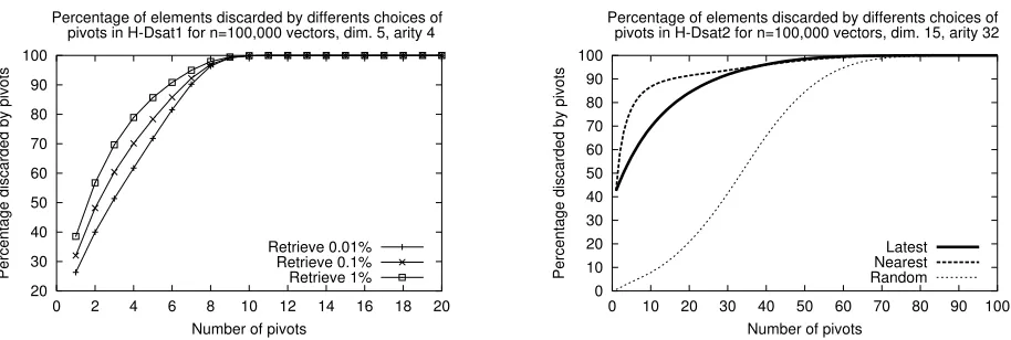
Because of the insertion process of H–DSAT1, the latest pivots of a node should be good since they are close, and hence good representatives, of the node. We verify experimentally that most discards using pivots were due to the latter ones. Figure 1 (left) shows that a small number of latter pivots per node suffices. In dimension 5, about 10 pivots per node discard all the elements that can be discarded using pivots. In higher dimensions, even less pivots are needed. We call H–DSAT1 k

Latest to this alternative.

20 30 40 50 60 70 80 90 100

0 2 4 6 8 10 12 14 16 18 20

Percentage discarded by pivots

Number of pivots

Percentage of elements discarded by differents choices of pivots in H-Dsat1 for n=100,000 vectors, dim. 5, arity 4

Retrieve 0.01% Retrieve 0.1% Retrieve 1%

0 10 20 30 40 50 60 70 80 90 100

0 10 20 30 40 50 60 70 80 90 100

Percentage discarded by pivots

Number of pivots

Percentage of elements discarded by differents choices of pivots in H-Dsat2 for n=100,000 vectors, dim. 15, arity 32

Latest Nearest Random

Figure 1: Percentage of elements discarded using the latest pivots in H–DSAT1 (left), and using the

The ancestors of a node are close to it, but the siblings of the ancestors are not necessarily close. So we expect that using the k latest pivots in H–DSAT2 (H–DSAT2 k Latest) does not perform as

well as before. An obvious alternative is H–DSAT2 k Nearest, which uses the k nearest pivots, not

theklatest. Figure 1 (right) confirms that less nearest pivots are needed to discard the same number

of nodes as latest pivots. However, note that for H–DSAT2 k Nearest we need to store the references

to the pivots in order to computeD. Hence, given a fixed amount of memory, this alternative must

use less pivots per node than the others.

We have introduced a parameterkin our data structures, which can be easily tuned since it depends

on the available memory. When k = 0the data structure becomes the originaldsa–tree, and when

k =1it becomes our unrestricted data structures of Section 4.

5.2

Choosing Good Nodes

The dual question is whether some tree nodes profit more from pivots than others. We experimentally study the features of the elements that are discarded using pivots. The result is that, for all the metric spaces used, the discarded elements are located near the leaves in the tree. In the vector space of dimension 5, the percentage varies from 40% to 60% (depending of the query radius), while in the space of dimension 15, almost the 100% of the elements discarded by pivots are leaves. In the dictionary this percentage varies from 80% to 90%.

The reason is that the covering radii of the nodes decrease as we go down in the tree, being zero in the leaves. As the covering radius infeasibility condition for a nodeaisD(a;q) > R (a)+r, the

probability of discardingaincreases whenR (a)decreases.

Suppose that we restrict the number of pivots per node to a value k. As leaves are discarded

more frequently than internal nodes, we consider an alternative that profits from this fact when using limited memory. The idea is to move the storage of pivots to the leaves smoothly and dynamically.

We have a parameter, which is0661. rhoallows us to determine the number of pivots per

node such that:(1)internal nodes havekpivots (unless they do not have so many to choose), and(2)

external nodes have all the pivots that the scheme permits (unless there is not enough available space). The way to implement this is as follows: When an external node becomes internal it retainsk of its

pivots, and it yields the others to the public repository, and when a new external node appears it takes from the repository all the pivots that it needs (whenever the repository has that many, in other case it takes all the available ones).

In this way, each new element attempts to take a number of pivots as close as possible to its original number of pivots, and memory usage tends to move dynamically to the leaves. The parameterallows

us to control the degree of movement of storage to the leaves. Note that when = 0, all the pivots

move to the leaves, and when=1the memory management has no effect.

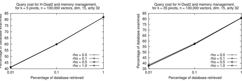
Figure 2 shows the experimental query cost for H–DSAT2 k Nearest, in the vector space of

di-mension 15, usingk = 5andk =35pivots, and values0,0:1, 0:5, and1for. In this metric space,

we get the best performance with=0.

6

Experimental Results

40 45 50 55 60 65 70 75 80 85

0.01 0.1 1

Percentage of database examined

Percentage of database retrieved Query cost for H-Dsat2 and memory management, for k = 5 pivots, n = 100,000 vectors, dim. 15, arity 32

rho = 0.0 rho = 0.1 rho = 0.5 rho = 1.0

35 40 45 50 55 60 65 70 75 80 85

0.01 0.1 1

Percentage of database examined

Percentage of database retrieved Query cost for H-Dsat2 and memory management, for k = 35 pivots, n = 100,000 vectors, dim. 15, arity 32

rho = 0.0 rho = 0.1 rho = 0.5 rho = 1.0

Figure 2: Performance of H–DSAT2 k Nearest with memory management, and various values of .

We selected values ofk =5pivots (left) andk =35pivots (right).

(minimum number of character insertions, deletions and substitutions to make the strings equal), of interest in spelling applications. The other spaces are real unitary cubes in dimensions 5 and 15 under Euclidean distance, using 100,000 uniformly distributed random points. We treat these just as metric spaces, disregarding coordinate information.

In all cases, we left apart 100 random elements to act as queries. The data structures were built 20 times varying the order of insertions. We tested arities 4, 8, 16, and 32. Each tree built was queried 100 times, using radii 1 to 4 in the dictionary, and radii retrieving 0.01%, 0.1%, and 1% of the set in vector spaces.

In [1] we show that H–DSAT1F outperformed H–DSAT1D, clearly in the dictionary and slightly

in vector spaces. The results are similar on H–DSAT2. Also we show experimentally that our struc-tures are competitive, as our best versions of H–DSAT1 and H–DSAT2 largely improve upon dsa– trees. This shows that our structures make good use of extra memory. H–DSAT2 can use more

memory than H–DSAT1, and hence its query cost is better.

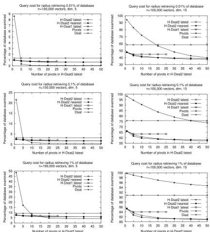
However, there is a price in memory usage, e.g., H–DSAT1 needs 1.3 to 4.0 times the memory of

dsa–tree, while H–DSAT2 requires 5.2 to 17.5 times. Hence the interest in comparing how well our

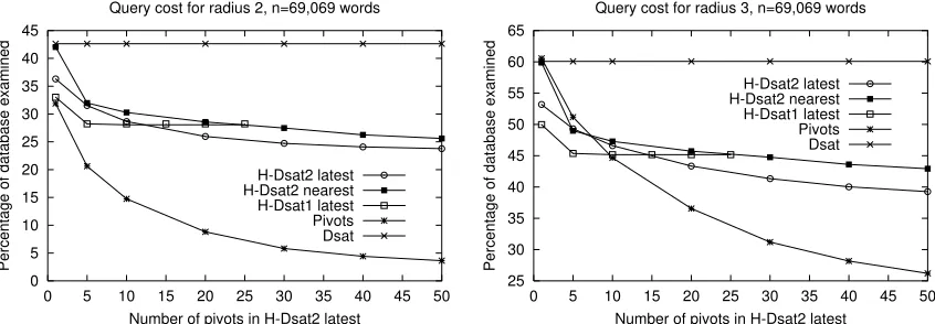
structures use limited memory compared to others. Figure 3 and Figure 4 compare against a generic pivot data structure, using the same amount of memory in all cases. We also show a dsa–tree as a reference point, as it uses a fixed amount of memory. In easy spaces (dimension 5 or dictionary) we do better when there is little available memory, but in dimension 15 H–DSAT2 is always the best. More pivots are needed to beat H–DSAT in harder problems.

7

Conclusions

0 1 2 3 4 5 6 7 8 9

0 5 10 15 20 25 30 35 40 45 50

Percentage of database examined

Number of pivots in H-Dsat2 latest Query cost for radius retrieving 0.01% of database

n=100,000 vectors, dim. 5

H-Dsat2 latest H-Dsat2 nearest H-Dsat1 latest Pivots Dsat 30 40 50 60 70 80 90 100

0 5 10 15 20 25 30 35 40 45 50

Percentage of database examined

Number of pivots in H-Dsat2 latest Query cost for radius retrieving 0.01% of database

n=100,000 vectors, dim. 15

H-Dsat2 latest H-Dsat2 nearest H-Dsat1 latest Pivots Dsat 0 5 10 15 20 25

0 5 10 15 20 25 30 35 40 45 50

Percentage of database examined

Number of pivots in H-Dsat2 latest Query cost for radius retrieving 0.1% of database

n=100,000 vectors, dim. 5

H-Dsat2 latest H-Dsat2 nearest H-Dsat1 latest Pivots Dsat 55 60 65 70 75 80 85 90 95 100

0 5 10 15 20 25 30 35 40 45 50

Percentage of database examined

Number of pivots in H-Dsat2 latest Query cost for radius retrieving 0.1% of database

n=100,000 vectors, dim. 15

H-Dsat2 latest H-Dsat2 nearest H-Dsat1 latest Pivots Dsat 0 5 10 15 20 25 30 35 40 45 50

0 5 10 15 20 25 30 35 40 45 50

Percentage of database examined

Number of pivots in H-Dsat2 latest Query cost for radius retrieving 1% of database

n=100,000 vectors, dim. 5

H-Dsat2 latest H-Dsat2 nearest H-Dsat1 latest Pivots Dsat 80 82 84 86 88 90 92 94 96 98 100

0 5 10 15 20 25 30 35 40 45 50

Percentage of database examined

Number of pivots in H-Dsat2 latest Query cost for radius retrieving 1% of database

n=100,000 vectors, dim. 15

H-Dsat2 latest H-Dsat2 nearest H-Dsat1 latest Pivots Dsat

Figure 3: Query cost of H–DSAT1F and H–DSAT2F versus a pivoting algorithm, in vector spaces.

We study the way to choose good pivots when the amount of memory is limited. Several alterna-tives are explored and evaluated.

In this paper we have also presented a method to delete elements from a hybrid dynamic spatial approximation tree. This method has shown to be better than that of the original method over a

dsa–tree.

dele-0 5 10 15 20 25 30 35 40 45

0 5 10 15 20 25 30 35 40 45 50

Percentage of database examined

Number of pivots in H-Dsat2 latest Query cost for radius 2, n=69,069 words

H-Dsat2 latest H-Dsat2 nearest H-Dsat1 latest Pivots Dsat

25 30 35 40 45 50 55 60 65

0 5 10 15 20 25 30 35 40 45 50

Percentage of database examined

Number of pivots in H-Dsat2 latest Query cost for radius 3, n=69,069 words

H-Dsat2 latest H-Dsat2 nearest H-Dsat1 latest Pivots Dsat

50 55 60 65 70 75 80

0 5 10 15 20 25 30 35 40 45 50

Percentage of database examined

Number of pivots in H-Dsat2 latest Query cost for radius 4, n=69,069 words

H-Dsat2 latest H-Dsat2 nearest H-Dsat1 latest Pivots Dsat

Figure 4: Query cost of H–DSAT1F and H–DSAT2F versus a pivoting algorithm, in the dictionary.

tions over arbitrarily long periods of time without any reorganization, and that can take advantage of available memory to improve search and deletion costs.

References

[1] D. Arroyuelo, F. Mu˜noz, G. Navarro, and N. Reyes. Memory–adptative dynamic spatial approx-imation trees. In Proceedings of the 10th International Symposium on String Processing and Information Retrieval (SPIRE 2003), LNCS. Springer, 2003. To appear.

[2] E. Ch´avez, G. Navarro, R. Baeza-Yates, and J.L. Marroqu´ın. Proximity searching in metric spaces. ACM Computing Surveys, 33(3):273–321, September 2001.

[3] G. Navarro and N. Reyes. Fully dynamic spatial approximation trees. InProceedings of the 9th International Symposium on String Processing and Information Retrieval (SPIRE 2002), LNCS 2476, pages 254–270. Springer, 2002.