RBF neural network implementation in hardware

RBF Neural Network Implementation in Hardware

Lucas Leiva 1 2_{, Nelson Acosta}1_,

1 _{INCA/INTIA Research Institute, UNICEN University}

Campus Universitario, Paraje Arroyo Seco (7000) Tandil, Bs. As., Argentina

2 _{CONICET - National Council of Scientific and Technological Research, Argentina}

{lleiva, nacosta}@exa.unicen.edu.ar

Abstract. This paper presents a parallel architecture for a radial basis function (RBF) neural network used for pattern recognition. This architecture allows defining sub-networks which can be activated sequentially. It can be used as a fruitful classification mechanism in many application fields. Several implementations of the network on a Xilinx FPGA Virtex 4 - (xc4vsx25) are presented, with speed and area evaluation metrics. Some network improvements have been achieved by segmenting the critical path. The results expressed in terms of speed and area are satisfactory and have been applied to pattern recognition problems.

Keywords: RBF neural network, FPGA, pattern recognition.

1 Introduction

Artificial neural networks are used as a modeling technique that emulates the human brain. The main characteristic of a neuronal network is its ability to learn internal features by through data sets analysis. A neuronal network is made of a set of simple processing units, each one with a natural capability to store experimentally acquired knowledge together with the ability to use them readily.

The neural networks may be classified in terms of the systems they are intended to be used for [1]. The networks used in pattern recognition processes maybe readily used for classification systems. Classification procedures involve the derivation of a function dedicated to split data into categories, defined from a set of features. This function is activated by a neuron-classifier, trained to use different types of input data along with their categories.

A classification network links any input vector to a well established category, producing an output signal identifying this category. Moreover, the network can set some level of input acceptance within the selected category. This means that the output is not just binary.

layer is responsible for producing the sum of the products obtained from the hidden layer weights (Fig. 1.).

Fig. 1. Radial Basis Function Neural Network

The hidden layer applies a function depending from the distance between the parametric charge vector (vi) and the input vector. These functions represent a special

class of functions whose main feature is a response decreasing with the increasing distance to the central point. A typical example is the Gaussian function.

Each radial basis function has an influence only in its receptive field, which is a small region of the featured space. The important regions of space are covered by a number n of functions.

Each radial basis function is attending to a small convex region called receptive field. A number of these functions cover a large space portion with their receptive fields. The output layer may thus associate some of them to regions with classes not linearly separable. Therefore, the number of RBF´s must be large enough to cover all subclasses that are linearly separable. Fig. 2 shows how the radial basis functions can cover any area of interest, no matter the shape of those regions.

Hardware Implementation of neural techniques has a significant number of advantages, mainly in the processing speed. For networks with large numbers of neurons and synapses, the conventional processors are not able to provide real time responses and training capacities, while parallel processing of multiple simple procedures achieves a large increase in speed.

Fig. 2. RBF Contour curves in 2D space.

.

.

1

2

n

.

.

1

j

.

.

x

x

x

1

j

.

.

v

v

v

Another advantage of implementing neural computing dedicated hardware is its ability to provide robust solutions for applications where it is not possible to install a PC. Such is the case for toys or autonomous robots for industrial uses or exploration. Numerous neural networks hardware implementation are available, such as the IBM ZISC78 device, Hitachi Digital Chip, Philips L-Neuro 1.0, Nestor Ni 100 [5] [6] [7], ZISC78[8], CM1K[9] devices.

The section 2 presents the hardware architecture of a RBF neural network implementation on a FPGA and section 3 analyzes the implementation in terms of area and speed. A several number of implementations were made, evaluating these parameters against the prototype size, the neurons number, and segmentation registers number. Finally, the section 4 describes the conclusions of this work.

2 Implementation

A neural network is made of a neuron set, each of them being associated with a category. Its operation basically begins with the occurrence of an input vector from which the neurons calculates the distance of this vector with the prototype stored in each of them. This prototype vector describes the "learning" of the neuron. The distance is compared with the influence field, which describes the receptive field. If the input vector lies in the neuron influence area, then the neuron is fired. Among the fired neurons, one is selected, with the shortest distance. The resulted category is then the one contained in this neuron.

Particular cases exist where the active (fired) neurons have different categories. In these cases, the network must indicate that the result is uncertain, as the system cannot determinate a confident response.

Given this behavioral description of a RBF neural network, this paper proposed an architecture which consists of a set of neurons and a controller responsible for coordinating the operations. Each neuron is composed of a prototype, a register which stores the influence field (NAIF), the category to which it belongs (CAT) and an additional register storing the distance (DST) between the feature vector and the stored prototype (Fig. 3). Both, the influence field and the category status are instantiated in VHDL code.

The function of distance is calculated allowing the following distance norms for the input feature vector (FV) and the prototype stored in the neuron (P):

L: DST = | FVi - Pi | (1)

LSUP: DST = Max( | FVi - Pi |) (2)

Fig. 3. Artificial neuron architecture.

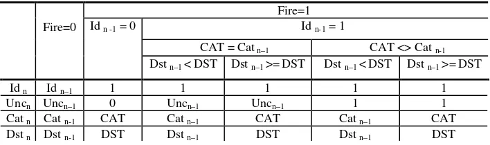
The inter-neural communication bus is composed by four signals. The first of them, indicates the pattern identification (Id), the next one indicates whenever a pattern has to be associated with two or more categories, making the classification uncertain (Unc). The other two signals consist of the smaller distance (Dst) together with the category (Cat) which involves this distance. Depending on the neuron state in front of an output enable signal, the bus controller behaves according to Table 1, where in-1 is an input bus signal while in is an output bus signal, i = {Id, Unc, Cat,

Dst}.

Table 1. Inter-neuron communication bus behavior.

Fire=1 Id n-1 = 1

CAT = Cat n–1 CAT <> Cat n-1

Fire=0 Id n -1 = 0

Dst n–1 <DST Dst n–1 >=DST Dst n–1 <DST Dst n–1 >=DST

Id n Id n–1 1 1 1 1 1

Uncn Uncn–1 0 Uncn–1 Uncn–1 1 1

Cat n Cat n-1 CAT Cat n–1 CAT Cat n–1 CAT

Dst n Dst n-1 DST Dst n–1 DST Dst n–1 DST

If the neuron is not fired, the input bus is mapped directly onto the output bus. However, if the neuron is fired the identification signal of the output bus will be 1 (Idn =1). On the other hand, if the input bus indicates an earlier identification (Idn-1 =

1) while the neuron is set active, an uncertainty arises about the equality between the category stored in the neuron and that of in the input bus. If they diverge, an uncertain signal will be activated on the output bus (Uncn = 1), otherwise the uncertainty output

will be that of the input (Uncn = Uncn-1). Actually, although no difference exists

between both inputs, the bus contains the category of smallest distance found, up to the moment some uncertainty is carried out.

load enable

out enable

Distance Function

Bus Control

< 0

1 . . .

fire

CAT DST NAIF

p

r

o

t

o

t

y

p

e

index

neuron com. bus

For the distance to the output bus, the controller simply verifies that the distance from the neuron (DST) is less than that of the input bus (Dstn). If so, the distance of

the output bus will be the one calculated by the neuron while the output category (Catn) wills the one that corresponds to the neuron. If the distance from the neuron is

greater than the input bus distance, these signals will be mapped along with the category of the output bus.

For the first neuron in the network, identification signal and uncertainty signal must be 0 while the distance must be the greatest possible (Table 1).

The interconnection neuron buses ease the linkage of several neurons in cascade.Those buses impose a critical path in what concerns the system design, directly associated with the number of neurons in the network. It is well known that these critical paths can be resolved through the use of registers, in such a way to divide paths with greater latency into shorter ones. For this sake, one proposes to include intermediate registers, uniformly distributed on the inter-neuron communication bus.

The controller allows the existence of multiple subnets to be triggered in serial form; In figure 4, net is the active subnet, nets_number the number of subnets contained, fv_count corresponds to the position vector with entries belonging to the subnet currently analyzed, fv_size(i) is the size of the ith subnet contained in the device, NR is the number of delay cycles (number of neuronal interconnection bus registers) needed to validate the output data of the inter- neuron communication bus and nc_count the actual delay cycle.

Fig. 4. Controller state machine.

The controller operational sequence is presented in Table 2, where (k) is the set of operations of the transition (k) of the preceding state machine, rej(i) is the reading

for the jth position of the characteristic vector, oej is the output enable signal, CATj

indicates the category storage and DSTj the stored distance, for the jth subnet. The

table shows an instruction overlap reducing the number of the required cycles for the operation.

Table 2. Controller operational sequence.

Cycle Re le oe DST CAT

0 re0(0) (1)

1 re0(1) le0(0)

… … …

N re0(N) le0(N-1)

(2) (2) (2)

N+1 re1(0) le0(N) (3)

N+2 re1(1) le1(0) oe0 (4)

... ... ... ... (5)

N+NR+2 re1(NR+1) le1(NR) oe0 (5)

N+NR+3 re1(NR+2) le1(NR+1) DST(0) CAT(0) (6)

N+NR+4 re1(NR+3) le1(NR+2) (2)

... ... ... (2)

N+M re1(M) le1(M-1) (2)

N+M+1 le1(M) (7)

N+M+2 oe1 (8)

… ... (9)

N+M+NR+2 oe1 (9)

N+M+NR+3 DST(1) CAT(1) (10)

There are so many control signals (oe, we, re) as subnets into the device. Assuming that a neural network contains multiple subnets, the number of cycles associated to its classification (CClassify), is given by:

C

= + +

r nets_numbe

0 j

) dim(

3 NR FVj (3)

where NR is the inter neuron communication bus registers number and FVj the

characteristic vector corresponding to the jth subnet. As it can be observed, the number of cycles is independent of the classification results.

This implementation does not support embedded (on-the-chip) learning. To carry out this feature it would be necessary to adopt a strategy for receptive field centers selection [10], incorporating a number of empty (untrained) neurons. Reconfigurable logic could be a valuable approach.

3 Experimental Results

composed by a single subnet. The prototype vectors stored in the neurons were generated randomly.

These architectures were implemented on Xilinx Virtex4 (xc4vsx25-11-ff668) FPGA [11]. The synthesis has been achieved with XST (Xilinx Synthesis Technology) [12] while the physical implementation used Xilinx ISE (Integrated Software Environment) version 7.1.04i [13], using default options in both cases. In this presentation no mention is made about the input data stream. These data can be stored in LUTs, block RAMs or external memory.

The behavior of an architecture without inter neuronal registers has been analyzed with different prototype vector sizes (16, 32, 64) in a range of 6 to 30 neurons. This size relies on the application field. It has been observed that the influence of the vector size is practically zero both on area (Fig. 5) and latency (Fig. 6).

0 500 1000 1500 2000

6 8 10 12 14 16 18 20 22 24 26 28 30 dim16

dim 32

dim 64

(neurons) (slices)

Fig. 5. Prototype vector size effect on area

0 20 40 60 80 100

6 8 10 12 14 16 18 20 22 24 26 28 30

dim 16 dim 32 dim 64 (ns)

(neurons)

Fig. 6. Prototype vector size effect on latency

# Slices ≅ 59.53 x Neurons + 54.57 (4)

Latency≅ 2.92 x Neurons + 2.019 (5)

The other important aspect to be looked at is the benefit of incorporating inter-neuron registers. A number of neural networks have been automatically generated with a number of neurons between 4 and 20, with prototype vector size fixed to 16, and inter-neuron registers number fixed to 0, 1 and 2. Fig. 8 and 9 display the results obtained in function of area and latency.

0 500 1000 1500 2000

6 8 10 12 14 16 18 20 22 24 26 28 30 Registers = 0

Registers = 1 Registers = 2

(neurons) (slices)

Fig. 7. Inter-neural registers effect on area

0 20 40 60 80 100

6 8 10 12 14 16 18 20 22 24 26 28 30 Registers = 0

Registers = 1 Registers = 2

(neurons) (ns)

Fig. 8. Inter-neural registers effect on latency

These figures show that the number of intermediate registers has a significant impact in both area and maximum operating frequency. Incorporating one inter-neuron register an 89% acceleration is achieved; incorporating two registers, the acceleration reaches 169% figure with respect to an unsegmented architecture.

0 1 2 3 4 5 6

4 6 8 10 12 14 16 18 20

M

il

li

o

n

s

dim 8 dim 16 dim 32 (Patterns/seg)

(neurons)

Fig. 9. Analysis of the dimension effect on the operating frequency

The ZISC78 devices needs at least feature vector size + 34 cycles to perform a classification, with 33 MHz clock frequency. This performance is constant with any number of neurons, being the maximum per chip of 78. The chip allows connecting multiple chips in chain to form greater neural networks. Comparing the performance obtained by the implementation and the ZISC78 devices, the implementation has a greater throughput at least for a small number of neurons (Fig. 10).

0 0,5 1 1,5 2 2,5 3 3,5

6 8 10 12 14 16 18 20 22 24 26 28 30

M

il

li

o

n

s

dim 16 dim 16 (ZISC) dim 32 dim 32(ZISC) (Patterns/sec)

(neurons)

Fig. 10. ZISC78 vs. implementation throughput

4 Conclusions

consumes a large portion of operating time. Better results can be obtained optimizing the characteristics extraction phase and incorporating a pipelining. The inter-neuron registers allowed an operating frequency of 50 MHz, impossible to achieve otherwise.

The comparison between this implementation and ZISC commercial chip demonstrates that this architecture is well suitable for application with small number of neurons demand.

Prospective future works will use this generated architecture in other areas of application (e.g. signals) and incorporate embedded learning.

Acknowledgments. The authors would like to thanks Géry Bioul for his support in the revision of this work.

References

1. Wolfram Research, Inc, “Neural Networks”, Wolfram Research, Inc, 2005

.

2. J. Moody and C. Darken, “Learning with localized receptive fields”, Proc. Connectionist Models Summer School, San Mateo, CA, 1988.

3. I. Park and I. W. Sandberg, “Universal approximation using radial basis function networks,” Neural Computat., vol. 3, pp. 246–257, 1991.

4. StatSoft Inc, “Neural Networks”, www.statsoftinc.com, 2003.

5. Valeriu Beiu, “Digital integrated circuit implementations”, Handbook of Neural Computation release 97/1, Publishing Ltd and Oxford University Press,1997.

6. Clark S. Lindsey , Bruce Denby , & Thomas Lindblad, “Neural Network Hardware”, http://neuralnets.web.cern.ch/NeuralNets/nnwInHep.html, 1998.

7. Yihua Liao, “Neural Networks in Hardware: A Survey”, Department of Computer Science, University of California, 2001.

8. Silicon Recognition, “ZISC: Zero Instruction Set Computer”, Version 4.2, Silicon Recognition, Inc., 2002

9. Z. Uykan, “Clustering-Based Algorithms for Radial Basis Function and Sigmoid Perceptron Networks,” Ph.D. dissertation, Control Eng. Lab.,Helsinki Univ. Technol., Helsinki, Finland, 2001.

10.Cognimem, CogniMem_1K: Neural network chip for high performance pattern recognition, datasheet, Version 1.2.1, www.recognetics.com, 2008.

11.Xilinx, Inc. Virtex-4 User Guide, UG070 (v2.6). www.xilinx.com, 2008.

12.Xilinx, Inc. Xilinx Synthesis Technology (XST) User Guide. UG627 (v 11.1.0) www.xilinx.com, 2009.

13.Xilinx, Inc. ISE 9.1.03i Documentation. www.xilinx.com, 2009.

14.L. Leiva, “Herramienta para Diseño Automático de Arquitecturas Basadas en Redes Neuronales para Reconocimiento de Patrones Visuales”, Graduation thesis, System Engineering, UNCPBA, 2006.