Author's personal copy On cycle-to-cycle heat release variations in a simulated spark ignition heat engine

(1)

Other uses, including reproduction and distribution, or selling or

licensing copies, or posting to personal, institutional or third party

websites are prohibited.

In most cases authors are permitted to post their version of the

article (e.g. in Word or Tex form) to their personal website or

institutional repository. Authors requiring further information

regarding Elsevier’s archiving and manuscript policies are

encouraged to visit:

(2)

On cycle-to-cycle heat release variations in a simulated spark ignition heat engine

P.L. Curto-Risso

a

, A. Medina

b,⇑,1

, A. Calvo Hernández

b,2

, L. Guzmán-Vargas

c

, F. Angulo-Brown

d a

Instituto de Ingenierı´a Mecánica y Producción Industrial, Universidad de la República, 11300 Montevideo, Uruguay b

Departamento de Física Aplicada, Universidad de Salamanca, 37008 Salamanca, Spain c

Unidad Profesional Interdisciplinaria en Ingenierı´a y Tecnologı´as Avanzadas, Instituto Politécnico Nacional, Av. IPN No. 2580, L. Ticomán, México D.F. 07340, Mexico d

Departamento de Fı´sica, Escuela Superior de Fı´sica y Matemáticas, Instituto Politécnico Nacional, Edif. No. 9 U.P. Zacatenco, México D.F. 07738, Mexico

a r t i c l e

i n f o

Article history: Received 30 July 2010

Received in revised form 19 October 2010 Accepted 19 November 2010

Available online 18 December 2010

Keywords:

Spark ignition engines Cycle-to-cycle variability Quasi-dimensional simulations Non-linear dynamics

a b s t r a c t

The cycle-by-cycle variations in heat release are analyzed by means of a quasi-dimensional computer simulation and a turbulent combustion model. The inﬂuence of some basic combustion parameters with a clear physical meaning is investigated: the characteristic length of the unburned eddies entrained within the ﬂame front, a characteristic turbulent speed, and the location of the ignition kernel. The evo-lution of the simulated time series with the fuel–air equivalence ratio,/, from lean mixtures to over stoi-chiometric conditions, is examined and compared with previous experiments. Fluctuations on the characteristic length of unburned eddies are found to be essential to simulate the cycle-to-cycle heat release variations and recover experimental results. A non-linear analysis of the system is performed. It is remarkable that at equivalence ratios around/’0.65, embedding and surrogate procedures show that the dimensionality of the system is small.

1. Introduction

Nowadays, primary objectives for vehicle manufacturers are the reduction of fuel consumption as well as the reduction of emissions. Among the several solutions to be adopted are fast com-bustion, lean burn, variable valve timing, gasoline direct injection, internal exhaust gas recirculation, and some others[1–3]. Combus-tion in spark-igniCombus-tion engines in lean burn condiCombus-tions can lead to cycle-to-cycle variations (CV) that are responsible for higher emis-sions and limit the practical levels of lean-fueling. Better models for simulating the dynamic character of CV could lead to new design and control alternatives for lowering emissions and expanding the actual operation limits.

The cyclic variation experienced by spark-ignition engines is essentially a combustion problem which is affected by many engine and operating variables like fuel properties, mixture com-position near spark plug, charge homogeneity, ignition, exhaust dilution, etc.[4]. Physical sources of CV arise from the merging of at least the following elements[5,6]:

(1) Motion of the gases mixture and turbulences during combustion.

(2) The amounts of fuel, air, and residual or recirculated exhaust gas in the cylinder.

(3) Homogeneity of the mixture composition, specially in the vicinity of the spark plug.

(4) Details of the spark discharge, like breakdown energy and the initial ﬂame kernel random position.

Not all these factors are equally important, and some others were not included in the list. It is usually argued that the first item in the list has the leading effect. The flow motion in any piston en-gine is unsteady, having an average pattern and a fluctuating veloc-ity component. Nevertheless, it is not easy to select an adequate turbulence parameter. During the engine operation not all the burnt gases are expelled from the combustion chamber in the ex-haust stroke. Some fraction is mixed with the next incoming air and fuel mixture in the following intake stroke. So, when combus-tion approaches the lean flammability limit, very small modifica-tions due to recycled gases in the mixture composition or temperature can greatly affect the next combustion event causing a highly non-linear cycle-to-cycle coupling process.

Besides experimental [6–12] and theoretical thermodynamic studies [13,14], computer simulations [14–16] are useful tools which provide complementary understanding of the complex physical mechanisms involved in the operation of a real engine. Several previous studies [6,17] tried to reproduce experimental CV by incorporating explicit models for ignition, combustion

⇑Corresponding author. Tel.: +34 923 29 44 36; fax: +34 923 29 45 84. E-mail addresses: pcurto@ﬁng.edu.uy (P.L. Curto-Risso), amd385@usal.es (A. Medina), anca@usal.es (A. Calvo Hernández), lguzmanv@ipn.mx (L. Guzmán-Vargas),angulo@esfm.ipn.mx(F. Angulo-Brown).

1

Present address: ETSII de Béjar, Universidad de Salamanca, 37700 Béjar, Salamanca, Spain.

2

Present address: IUFFYM, Universidad de Salamanca, 37008 Salamanca, Spain.

Contents lists available atScienceDirect

Applied Energy

(3)

chemistry, flame evolution, and turbulence. In these models some input parameters are varied in each cycle in such a way that cycle-to-cycle combustion also changes, and so do the pressure and temperature in the cylinder and subsequently heat release, power output and efficiency. Abdi Aghdam et al.[6]reproduced satisfactory fits to pressure and flame radius data by performing quasi-dimensional computer simulations and acting on the rms turbulent velocity.

In regard to CV phenomenology we mention the following experimental and theoretical works, many of them related to the non-linear dynamics involved in these variations. Letelier et al.

[18]reported experimental results for the variation of the in-cylin-der pressure versus crank angle for a four-cylinin-cylin-der spark heat engine. By reconstructing the phase space and building the Poin-caré sections it was concluded that CV is not governed by a chaotic process but rather by a superimposition of a non-linear determin-istic dynamics with a stochastic component. In the works by Daw et al.[19,20], a physically oriented simple mathematical model was reported for the spark-ignition engine. The fuel/air mass ratio in a cycle was modeled as stochastic through random noise and non-linear deterministic coupling between consecutive engine cy-cles. The predicted CV trends for heat release versus fuel–air ratio were compared with experimental results by analyzing bifurcation plots and return maps for different parameters of the model (the mean fuel–air ratio, its standard deviation, and the fraction of the un-reacted air and fuel remaining in the cylinder). Also, an analysis of the temporal irreversibility in time-series measurements was presented by using a symbolic approach to characterize the noisy dynamics[21].

Litak and coworkers[10,22,23] have reported extensive work relative to cycle-to-cycle variations of peak pressure, peak pressure location and heat release in a four-cylinder spark ignition engine in terms on spark advance angle and different torque loadings under near-stoichiometric conditions. The observed qualitative change in combustion was analyzed using different statistical methods as re-turn maps, recurrence plots[22,24], correlation coarse-grained en-tropy[25]and, recently, multifractal techniques[23,26], and the so-called multi-scale entropy (MSE) (or sample entropy)[11]: an improved statistical tool to account for complexity measure in time series with multiple temporal or spatial scales. Recently, our group have applied monofractal and multifractal methods to char-acterize the ﬂuctuations for several fuel–air ratio values, from lean mixtures to stoichiometric situations[27]. For intermediate mix-tures a complex dynamics was observed, characterized by a cross-over in the scaling exponents and a broad multifractal spectrum.

Among simulation approaches to internal combustion engines, multi-dimensional models are based on the numerical solution of a set of governing coupled partial-differential equations, which are integrated in 2D or 3D geometric grids in the combustion cham-ber space[28–30]. Although these models provide very realistic information with spatial and temporal resolution, they demand large storage capacity and large computer times, particularly in cyc-lic variability problems. These drawbacks are avoided by quasi-dimensional models that improve zero-quasi-dimensional or thermody-namic models with the assumption of a spherical ﬂame front and the incorporation of two differential equations for combustion which describe the combustion evolution[28,31]. Thus, within rea-sonable computer times these models allow to investigate the main physical effects that cause cycle-to-cycle variations[6].

A main goal of this paper is to analyze the effect of some combustion parameters and their consequences on cycle-to-cycle variations of heat release for fuel–air equivalence ratios ranging from very lean mixtures to stoichiometric conditions. To this end we developed a quasi-dimensional computer simulation that incorporates turbulent combustion and a detailed analysis of the involved chemical reaction that includes in a natural way the

pres-ence of recycled exhaust gases in the fresh fuel–air mixture and valves overlapping. The model, previously developed and validated

[14], allows for a systematic study of the inﬂuence on CV of three basic combustion parameters: the characteristic length of the un-burned eddies, the characteristic turbulent speed, and the location of the ignition site. Our simulations correctly reproduce the basic statistical parameters for the fuel ratio dependence of experimen-tal heat release time series[20,26]. Moreover, we shall employ some standard techniques from non-linear data analysis in order to characterize our results and compare them with those from other authors: ﬁrst-return maps, bifurcation-like plots, and embedding and surrogate techniques to obtain the correlation dimension.

2. Simulated model: basic framework

We make use of aquasi-dimensionalnumerical simulation of a monocylindrical spark-ignition engine, previously described and validated[14]. Opposite tozero-dimensional(or thermodynamical) models where all thermodynamic variables are averaged over a fi-nite volume and an empirical correlation is used to approximate the combustion process, within the quasi-dimensional scheme ex-plicit differential equations are considered to solve combustion un-der the hypothesis of a spherical flame front. In our simulation model two ordinary differential equations are solved in each time step (or each crankshaft angle) for the pressure and the temperature of the gases inside the cylinder. This set of coupled equations (that are explicitly written in[14,15,32]) are valid for any of the different steps of the engine evolution (intake, compression, power stroke, and exhaust) except combustion. For this stage a two-zone model discerning between unburned (u) and burned (b) gases that are sep-arated by an adiabatic flame front with negligible volume is consid-ered. Thus, the temperature equation splits in equations forTuand

Tb. Moreover, differential equations giving the evolution of the

un-burned and un-burned mass of gases should be solved. Next we detail the main assumptions of the combustion model considered.

2.1. Combustion process

The ﬂame kernel development is the most important phase for the overall cyclic dispersion in the engine performance. For simu-lating combustion we assume the turbulent quasi-dimensional model (sometimes callededdy-burningorentrainmentmodel) pro-posed by Blizard and Keck[33,34]and improved by Beretta et al.

[35], by considering a diffusion term in the burned mass equation as we shall see next. The model starts from the idea that during ﬂame propagation not all the mass inside the approximately spher-ical ﬂame front is burned, but there exist unburned eddies of typ-ical lengthlt. Thus, a set of coupled differential equations for the

time evolution of total mass within the ﬂame front,me(unburned

eddies plus burned gas) and burned mass,mb, is solved:

_

mb¼

q

uAfSlþ

memb

s

b

ð1Þ

_

me¼

q

uAfut1et=sbþSl ð2Þ

At the beginning of combustion in each cycle an initial standard vol-ume for the ﬂame kernel is considered[36]. In the modelutis a

characteristic velocity at which unburned gases pass through the ﬂame front,

q

uis the unburned gas density, andAfis the ﬂame front

area.

s

bis a characteristic time for the combustion of the entrained

eddies,

s

b=lt/SlandSlis the laminar combustion speed that is

deter-mined from its reference value,Sl,0, as[37]:

Sl¼Sl;0

Tu

Tref

a

p pref

b

12:06y0:77 r

(4)

whereyris the mole fraction of residual gases in the chamber and

a

andbare functions of thefuel/air equivalence ratio,/[38]. The ref-erence laminar burning speed,Sl,0, at reference conditions (Tref,pref)

is obtained from Gülder’s model[39,38]. Because of the reasons that we shall present later, it is important to stress that the laminar speed, apart from the thermodynamic conditions, depends on the fuel/air equivalence ratio and on the mole fraction of gases in the chamber after combustion. Thus, Eq. (3)shows the coupling be-tween combustion dynamics and the residual gases in the cylinder after the previous combustion event. In other words, laminar burn-ing speed depends on the memory of the chemistry of combustion. From Eq.(2)it is easy to see that

s

bdetermines the time scale

asso-ciated either to the laminar diffusive evolution of the combustion at a velocitySlor to the rapid convective turbulent component

associ-ated tout.

In order to numerically solve the differential equations for masses (Eqs.(1) and (2)), it is necessary to determineAf,ut, andlt.

The ﬂame front area,Af, is calculated from the ﬂame front radius,

considering a spherical ﬂame propagation in a disc shaped combus-tion chamber[34]. The radius is calculated through the enﬂamed volume,Vf, following the procedure described by Bayraktar[40],

Vf ¼

mb

q

b

þmemb

q

u

ð4Þ

The ﬂame front area depends on the relative position of the kernel of combustion respect to the cylinder center, Rc, which have its

nominal value at the spark plug position, but convection at early times can produce signiﬁcant displacements. Forutandlt, Beretta

et al.[35]have derived empirical correlations in terms of the ratio between the fresh mixture density at ambient conditions,

q

i, and

the density of the unburned gases mixture inside the combustion chamber,

q

u:

ut¼0:08ui

q

u

q

i 1 2

ð5Þ

lt¼0:8Lv;max

q

i

q

u 3 4

ð6Þ

whereuiis the mean inlet gas speed, andLv, maxthe maximum valve

lift. Eqs.(1) and (2)must be solved simultaneously together with the set of differential equations for temperature and pressure

[14]. Respect to the end of combustion, we assume that if exhaust valve opens before the completion of combustion, it ﬁnishes at the moment of the opening.

Among the parameters that determine the development of combustion, there are three essential ones: the characteristic length of eddies lt(associated to the characteristic time,

s

b), the

turbulent entrainment velocityut(essential for the slope ofme(t)

during the fastest stage of combustion), and also Afor the ﬂame

radius centerRcthat gives the size and geometry of the ﬂame front

(and thus inﬂuences all process). Therefore, all these parameters could have strong inﬂuence on cycle-by-cycle variations.

In order to calculate the heat release during combustion we ap-ply the ﬁrst law of thermodynamics for open systems separating heat release,dQr, internal energy variations associated to

tempera-ture changes,d U, work output,dW, and heat transfers from the working ﬂuid (considered as a mixture of ideal gases) to the cylin-der walls,dQ‘:

dQr¼dUþdWþdQ‘ ð7Þ

where internal energy and heat losses include terms associated to either unburned or burned gases: U=mucv,uTu+mbcv,b Tb and

dQ‘=dQ‘,u+dQ‘,b. All these terms can be derived in terms of time

or of the crankshaft angle. Net heat release during the whole com-bustion period is calculated from the integration of heat release var-iation during that period. A particular model to evaluate heat

transfer through cylinder walls should be chosen before the numer-ical obtention ofQr. Units used throughout the paper are

interna-tional system of units except when explicitly mentioned.

2.2. Heat transfer

Among the different empirical models that can be found in the literature for heat transfer between the gas and cylinder internal wall we shall utilize that developed by Woschni[41],

_ Q‘

AtðTTwÞ

¼129:8p0:8_w0:8_B0:2_T0:55 _ð8Þ

whereAtis the instantaneous heat transfer area,pis the pressure

inside the cylinder,Tthe gas temperature,Twthe cylinder internal

wall temperature, Bthe cylinder bore, andwthe corrected mean piston speed[28]. All units are in the international system of units, except pressures which are in bar.

2.3. Chemical reaction

In order to solve the chemistry and the energetics of combus-tion we assume the unburned gas mixture as formed by a standard fuel for spark ignition engines (iso-octane, C8H18), air, and exhaust

gases. Exhaust chemical composition appears directly as calculated from solving combustion. The considered chemical reaction is,

ð1yrÞ½C8H18þ

a

ðO2þ3:773 N2Þ

þyr brCO2þ

c

rH2Oþ

l

rN2þ

m

rO2þ

e

rCOþdrH2þ þnrH

þ

j

rOþ

r

rOHþ

1

rNO !bCO2þ

c

H2Oþ

l

N2þ

m

O2

þ

e

COþdH2þ þnHþ

j

Oþ

r

OHþ

1

NO ð9Þ

where the subscriptrrefers to residual. We make use of the subrou-tine developed by Ferguson [42] (but including residual gases among the reactants) to solve combustion and calculate exhaust composition. Our model does not consider traces of C8H18in

com-bustion products, but in the energy release we actually take into account combustible elements as CO, H, or H2. The thermodynamic

properties of all the involved chemical species are obtained from the constant pressure speciﬁc heats, that are taken as 7-parameter temperature polynomials[43].

As a summary of the theoretical section it is important to note that in our dynamical system the coupled ordinary differential equations for pressure and temperature are in turn coupled with two other ordinary differential equations for the evolution of the masses during combustion. So, globally this leads to a system of differential equations where apart from several parameters (mainly arising from the geometry of the cylinder, the chemical reaction and the models considered for other processes), there is a large number of variables: pressure inside the cylinder,p, tem-peratures of the unburned and burned gases,Tu, andTb, and masses

of the unburned and burned gases,muandmb. All these variables

evolve with time or with the crankshaft angle. So, up to this point, our dynamical model is a quite intricate deterministic system with those time dependent variables.

3. Results

(5)

The computed results for heat release,Qr, for each of the ﬁrst

200 cycles are presented in Fig. 1a for a particular value of the fuel–air equivalence ratio, /= 1.0. This time evolution was ob-tained directly from the solution of the deterministic set of differ-ential equations. The curve clearly shows, after a transitory period, a regular evolution that does not match with previous experimen-tal studies of cycle-to-cycle variability on heat release[20,22]. For other equivalence ratios the curves obtained present different lev-els of variability but never display the typical experimental ﬂuctu-ations. So, the variability obtained by the direct solution of the non-linear deterministic set of equations for temperatures and pressures, and the evolution of masses during combustion seems not enough to reproduce the features of cyclic variability shown by experiments.

In order to analyze these time series we show inTable 1for sev-eral fuel ratio values, some usual statistical parameters: the aver-age value

l

, the standard deviation

r

, the coefﬁcient of variation,

COV=

r

/

l

, the skewness S¼PNi¼1ðxi

l

Þ3=½ðN1Þ

r

3, and the

kurtosisK¼PNi¼1ðxi

l

Þ4=½ðN1Þ

r

4.Sis a measure of the lack

of symmetry in such a way that negative (positive) values imply the existence of left (right) asymmetric tails longer than the right (left) tail.Kis a measure of whether the data are peaked (K> 3) or ﬂat (K< 3) relative to a normal distribution.

With the objective to recover the experimental results on cyclic variability we have checked the inﬂuence of incorporating a

stochastic component in any of the physically relevant parameters of the combustion model. We ﬁrst analyze the inﬂuence of the characteristic lengthltand velocityutkeeping the location of

igni-tion at the spark plug posiigni-tion (i.e., Rc= 25103m [35]).

Although both parameters can be considered as independent in our model (see below), we assume that they are linked by the empirical relations(5) and (6). We ﬁtted the experimental results by Beretta et al.[35]forltconsidered as a random variable to a

log-normal probability distribution,LogNð

l

loglt;

r

logltÞ, around the

nominal valuel0_t ¼0:8Lv;maxð

q

i=

q

uÞ

3=4_(Eq.₍₆₎_{) with standard}

devi-ation

r

loglt¼0:222 and mean

l

loglt¼logðl

0

tÞ ð

r

2loglt=2Þ. Then, in

each cycleutis obtained from Eq.(5)through the empirical

densi-ties ratio. It is worth-mentioning that the experiments by Beretta in[35]are directly results on the evolution of pressure during com-bustion with high-speed motion picture records of ﬂame propaga-tion. So, we ﬁtlt with experiments on combustion and tried to

recover cycle-to-cycle ﬂuctuations by adding an stochastic behav-ior of a key parameter of combustion on the deterministic simulation.

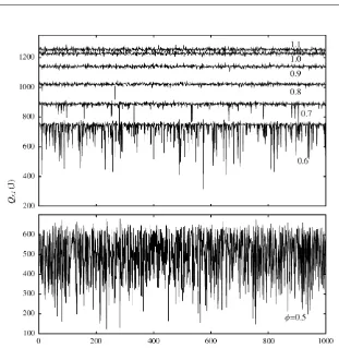
For several values of/ranging from very lean mixtures to over stoichiometric,Table 2shows the characteristics of the time evolu-tion of the heat release when the stochastic component onlthas

been introduced.Fig. 1b displays a time series for the stochastic computations at least qualitatively much similar to the experimen-tal ones in contrast to the deterministic for/= 1.0. It is important

1210 1220 1230 1240 1250

0 50 100 150 200

Qr

(J)

Cycles

(a)

[image:5.595.151.439.81.360.2]

(b)

Fig. 1.(a) Heat release time series as obtained from the simulation without the consideration of any stochastic component for/= 1.0. (b) Heat release time series,Qr,

[image:5.595.35.553.438.502.2]

obtained with a log-normal distribution (see text) for the characteristic length for unburned eddies during combustion,lt.

Table 1

Statistical parameters of the heat release temporal series, considering the deterministic model, for several fuel ratio values: mean value,l, standard deviation,r, coefﬁcient of covariance,COV, skewness,S, and kurtosis,K.

/ 0.5 0.6 0.7 0.8 0.9 1.0 1.1

l(J) 500.84 746.19 886.82 1019.73 1138.79 1227.20 1253.32

r(J) 2.593 0.320 0.785 1.463 1.969 2.249 2.255

COV(103

) 5.177 0.428 0.885 1.435 1.729 1.832 1.799

S 0.004 0.057 0.106 0.013 1.317 0.376 0.062

(6)

to note that it is difﬁcult to perform a direct quantitative compar-ison with experiments, because of the large number of geometric and working parameters of the engine[14], usually not speciﬁed to the full extent in the experimental publications.

From a comparison betweenTables 1 and 2, it is clear that aver-age values are of course similar, but the standard deviation and coefficient of variation are much smaller in the deterministic case. The behavior of skewness is subtle, it only could be concluded that globally in the deterministic case values forS are closer to zero (that would be the value corresponding to a Gaussian distribution). For the stochastic simulation kurtosis in the fuel ratio interval be-tween /= 0.6 and 0.8 is much higher than in the deterministic case, that is a sign of more peaked distributions.Fig. 2shows the evolution of heat release with the number of cycles for fuel ratios between 0.5 and 1.1. A careful inspection shows that at low and intermediate fuel-ratios distributions are quite asymmetric with tails displaced to the left. In other words, there exist remarkable poor combustion or misfire events. This is quantified by the evolu-tion with/of the skewness compiled inTable 2: it takes high neg-ative values in the interval /= 0.5–0.8. These results are in accordance with the experimental ones by Sen et al. [26] (see

Fig. 1in that paper).

We represent inFig. 3the evolution with the fuel–air equiva-lence ratio of the statistical parameters contained inTables 1 and

2in order to perform a direct comparison with previous experi-mental results. Although the experiments by Daw et al. [20,26]

were performed for a real V8 gasoline engine with a different cyl-inder geometry that the considered in our simulations, the depen-dence on / of the standard deviation, coefﬁcient of variation, skewness and kurtosis is very similar, although, of course, vertical scales in simulations and experiments are different. It makes no sense, to compare the mean values of heat release because of dif-ferent shape and size of the real and the simulated engine. It is clear from the ﬁgure that at intermediate fuel ratios, around, / = 0.7, skewness also reproduces a pronounced minimum and kur-tosis a sharp maximum. Nevertheless, our deterministic heat re-lease computations do not reproduce neither the evolution with / shown by experiments nor the magnitude of those statistical parameters.

Fig. 4represents the ﬁrst-return maps,Qr,i+1versusQr,i, for the

same values of/obtained from the deterministic simulation (dark points) and also from the stochastic computations (color points). Return maps when ltdoes not have a stochastic component, for

any value of fuel ratio, seem noisy unstructured kernels. Whenlt

[image:6.595.42.564.109.172.2]

is considered as stochastic a rich variety of shapes for return maps is found, depending on the fuel ratio. From the stochastic return maps in this ﬁgure and the statistical results inTable 2we stress the following points. First, at high values of/(0.91.1) variations Table 2

Statistical parameters of the heat release temporal series represented inFig. 2and obtained considering stochastic ﬂuctuations inlt, for several fuel ratio values.

/ 0.5 0.6 0.7 0.8 0.9 1.0 1.1

l(J) 492.50 726.23 885.43 1020.24 1139.51 1227.16 1253.71

r(J) 122.966 57.872 17.937 7.333 6.326 6.663 7.093

COV(103

) 250.0 79.7 20.3 7.2 5.6 5.4 5.7

S 0.643 3.028 8.388 3.194 0.147 0.423 0.335

[image:6.595.146.457.167.486.2]

K 2.495 13.455 104.475 49.491 3.579 3.710 3.454

Fig. 2.Heat release time series,Qr, obtained with a log-normal distribution (see text) for the characteristic length of unburned eddies during combustion,lt. Results are shown

(7)

of heat release behave as smallnoisyspots characteristic of small amplitude distributions with asymmetric right tails and slightly more peaked near the mean than a Gaussian distribution. For/ = 1.0 and 1.1 those noisy spots are partially overlapped. These re-sults are very similar to the experimental ones by Daw et al. (see

Fig. 1in[44]) for different engines and those by Litak et al. (see

Fig. 4in[22]). Second, at intermediate fuel ratios (/= 0.60.8) ex-tended boomerang-shaped patterns are clearly visible. Note that these series lead to distributions that are very peaked near the mean and decline rather rapidly, and have quite asymmetric left

tails. In this interval our results also are in accordance with those of Daw et al. [20,44]. Third, at the lowest equivalence ratio, / = 0.5 a change of structure is observed, probably because of cycle misﬁres for this very poor mixture. Here the probability distribu-tion is less peaked than a Gaussian, present a high standard devia-tion, and an asymmetric left tail. Fourth, a closer inspection of

Fig. 4reveals some kind of asymmetry around the diagonal, more pronounced as the fuel–air ratio becomes lower. This is in accor-dance both with experimental and model results by Daw et al.

[19,20,44]. So, our stochastic scheme with the consideration of 10

20 30 40 50 60 70 σ

Experimental

Ref. [26]

Simulated

0.05 0.10 0.15 0.20 0.25 0.30

CO

V

- 3.5 - 3.0 - 2.5 - 2.0 - 1.5 - 1.0 - 0.5 S

0.5 0.6 0.7 0.8 0.9 1.0

0 5 10 15 20

K

φ φ

20 40 60 80 100 120

0.05 0.10 0.15 0.20 0.25

-8 -6 -4 -2 -0

0.5 0.6 0.7 0.8 0.9 1.0

[image:7.595.55.529.83.630.2]

0 20 40 60 80 100

(8)

pseudo-random ﬂuctuations onltreproduces the characteristic

re-turn maps of this kind of systems from poor mixtures to over stoi-chiometric ones.

The results above refer to the joint inﬂuence of the parameters

utandlton the CV-phenomena when both parameters are

consid-ered linked by the empirical relations according to Eqs.(5) and (6). From now on our goal is two-fold: on one side, to analyze the inﬂu-ence ofutandltbut considered as independent in the simulation

model and, on the other side, to analyze the inﬂuence of the third key parameter in the combustion description, the location of igni-tion accounted for the parameterRc. To get this we have run the

simulation for 2800 consecutive cycles for the previously consid-ered fuel–air equivalence ratios but taking these three parameters, one-by-one, as stochastic in nature.

First, we have considered only ﬂuctuations on lt, taking the

same distribution as that in the beginning of this section. We show the corresponding return maps inFig. 5a, that should be compared withFig. 4. From this comparison we can conclude that the main characteristics of the return maps obtained when ltand utwere

considered as linked (noisy spots near-stoichiometric conditions, boomerang-shaped structures at intermediate fuel–air ratios and complex patterns at lower air–fuel ratios) are already induced by the distribution of the characteristic length lt when the other

parameters are not stochastic. Differences between both ﬁgures only affect the dispersion of the boomerangs arms.

In regard tout, it is important that it is not easy to ﬁnd in the

literature experimental data which allow to deduce stochastic dis-tributions for this characteristic turbulent velocity with certainty. We have used the data in [6] for the turbulence intensity and translated them to generate our log-normal distribution for the characteristic velocity,ut, and checked slight changes in the

distri-bution parameters within realistic intervals. So, we assume a log-normal distribution LogNð

l

logut;

r

logutÞaround the nominal value u0

t¼0:08uið

q

u=

q

iÞ 1=2

[Eq. (5)] with standard deviation

r

logut¼

0:02u0

t and mean

l

logut¼logðu

0

tÞ ð

r

2logut=2Þ. Whenutis the only

stochastic parameter, the observed behaviors are not signiﬁcantly altered (Fig. 5b): boomerang-like arrangements are found only at low/, although some sensitivity in the arms of the boomerangs is appreciable. Moreover, we have not found in the return maps new features with respect to those generated withlt.

Respect to the ignition location,Rc, some authors[45]concluded

from experiments and models that displacement of the ﬂame ker-nel during the early stages of combustion has a major part in the

origination of cycle-by-cycle variations in combustion. So, it seems interesting to check this point from quasi-dimensional simulations. It is remarkable that it is not straightforward to numerically evalu-ate the radius and area of the ﬂame front whenRcis displaced

respect to the origin. We have generalized the studies by Bayraktar

[46]and Blizard and Keck[34]to obtain numerical expressions for the radius and area of the ﬂame front for whichever value ofRcand

at any time during ﬂame evolution. Second, we assume a Gaussian distribution with standard deviation

r

Rc¼2:96510

3

m, accord-ing to the results reported by Beretta[35]. At sight ofFig. 5c it is clear that the inﬂuence of a stochastic component inRcis limited

to cause noisy spots at any fuel ratio, clear structures as boomer-angs are not found at any fuel–air equivalence ratio. So, fluctuations on the displacement of the initial flame kernel does not seem suffi-cient to reproduce characteristic patterns of CV.

Finally, we have checked what happens when the three param-eters are simultaneously and independently introduced as stochas-tic in the simulations with the distributions mentioned above and no new features were discovered. In view of these results we can say that the observed heat release behavior in terms of the fuel– air ratio is mainly due to stochastic and non-additive variations ofltandutand the non-linearity induced by the dynamics of the

combustion process, independently of ignition location ﬂuctuations.

Some physical consequences of cyclic variability are amenable of a clear interpretation in terms of the evolution of the fraction of burned gases in the chamber with time or with crank angle. This evolution has two main ingredients: the ignition delay (the inter-val until this fraction departs from zero)[18]and the slope of that increase during combustion (see, for instance, Fig. 16 in [35]). These factors are mainly associated to the length of characteristic eddiesltandut, and the laminar speedSl(that in turn is a function

of the fraction of residual gases,yr, in the chamber, Eq.(3)). This

last variable determines the memory effects from cycle-to-cycle, as noted by Daw et al.[19,20]. Cyclic variability provokes cycle-to-cycle changes in the shape of the rate of burned gases, and this directly affects the evolution of pressure during the cycle, particu-larly its maximum value and its corresponding position. Conse-quently this leads to changes in the performance of the engine, i.e., in the power output and in the efﬁciency.

4. Non-linear analysis: Correlation integral and surrogates

In accordance with the conclusions of the preceding section, all the results we present were obtained by considering ﬂuctuations only onlt, except when simulations were purely deterministic. In

order to get a better insight into the complexity of heat release fluctuations for different fuel ratio values, we next explore the non-linear properties of the signals through the analysis of the correlation integral [47–49]. The correlation dimension analysis quantifies the self-similarity properties of a given sequence and is an important statistical tool which helps to evaluate the pres-ence of determinism in the signal. We first reconstruct an auxiliary phase space by an embedding procedure. The correlation sum

Cð

e

;mÞ ¼2=½NðN1ÞPNi¼1

PN

j¼iþ1Hð

e

k~xi~xjkÞ, where H is the

Heaviside function,

e

is a distance and~xkarem-dimensional delay

vectors, is computed for several values of m and

e

[50]. If

C(

e

,m)/

e

d_{, the correlation dimension is deﬁned as} _d₍

_e

_{) =}_d_log

[image:8.595.51.285.89.271.2]

C(

e

,m)/dlog

e

. To get a good estimation ofm we need to repeat the calculations for several values ofm, the number of embedding dimensions. In this way we are able to select which one corre-sponds to the best option to characterize the dimensionality of the system. We notice that the application of correlation dimen-sion analysis alone is not sufﬁcient to differentiate between deter-minism and stochastic dynamics. To reinforce our calculations of

Fig. 4. Heat release return maps after 2800 simulation runs for the same values of/

(9)

correlation integral statistics, we consider a surrogate data method to verify that low values of correlation dimension of sequences are not a simple consequence of artifacts[51]. To this end, two surro-gate sets were considered. First, the original sequence was ran-domly shufﬂed to destroy temporal correlations. A second surrogate set was constructed by a phase randomization of the ori-ginal sequence. The phase randomization was performed after applying the Fast Fourier Transform (FFT) algorithm to the original time series to obtain the amplitudes. Then the surrogate set was obtained by applying the inverse FFT procedure[51,52].

We apply the correlation dimension method to heat release se-quences with 104

cycles and for different values of the fuel ratio in the interval 0.5 </< 0.7. For larger fuel ratios we disregard the correlation dimension analysis since the signal shows small ampli-tude ﬂuctuations around a stable value. According with the map-like characteristics observed inFig. 4we use a delay time equal to one.Fig. 6shows the correlation sum for two selected values of fuel ratio. We observe that for low values of/(/= 0.5,Fig. 6a) the correlation integral shows a power law behavior against

e

for several values ofm. This behavior is best found by plotting the sloped(

e

) of log(

e

,m) vs. log

e

. The inset shows this plot for values ofmin the range 1–5. In this case there is a wide plateau of

e

which corresponds to the power law behavior. It is also clear that the height of the plateau increases with the embedding dimension with a reduction of amplitude of the power law region and some ﬂuctuations for low values of

e

.

In contrast, we observe inFig. 6b that for intermediate fuel ra-tios (/= 0.65) the scaling region only exists for values of

e

in the

range 10 <

e

< 102_{. This is conﬁrmed by the presence of a plateau}

for several values ofm(see the inset inFig. 5b). Remarkably, the height of the plateau, d(

e

), almost does not change with the embedding dimension, indicating that the system can be charac-terized by a very low dimension. We also notice that for very small scales (

e

< 10), a power law behavior can be also identiﬁed, but the scaling exponent increases to reach the value of the embedding dimension, suggesting to identify this region as a noisy regime.

Next, we use the surrogate data method to evaluate if the low value of correlation dimension observed for/= 0.65 is not an arti-fact. We generated a randomly shufﬂed sequence and another set by a phase randomization of the original data. For both surrogate sets the correlation dimension was calculated in the same form and intervals as for original data. The results of these calculations are presented inFig. 7. We observe that for shufﬂed and phase ran-domized data the correlation dimension increases as the value ofm

also increases, indicating that there is no saturation for correlation dimension (Fig. 7a and b).

The ﬁndings about correlation dimension of original and surrogate data are summarized in the plots ofFig. 7c. For low fuel ratio values, the correlation dimension does not saturate for high embedding values whereas for the intermediate fuel ratio (/= 0.65), correlation dimension saturates with the embed-ding dimension which is an indication of low dimensional dynamics. It is also interesting that when ﬂuctuations onlt are

not included in the simulations (deterministic case) the same sit-uation is observed. The results for surrogate data (shufﬂed and phase randomized) reveal that no saturation of correlation 200

400 600 800 1000 1200 400 600 800 1000 1200 400 600 800 1000 1200

200 400 600 800 1000 1200

Qr

,

i

+

1

(J)

Qr,i(J)

φ

=0.5

0.6 0.7

0.8 0_.9

1.0 1.1 0.5

0.6 0.7

0.8 0.9

1.0 1.1 0.5

0.6 0_.7

0.8 0.9

1.0

1.1

(a)

(b)

[image:9.595.151.442.82.442.2]

(c)

Fig. 5.Heat release return maps obtained when the three basic parameters of combustion,lt,ut, andRcare considered as independent and one-by-one stochastic. (a)

(10)

dimension is observed, indicating that surrogate sequences differ from the original data and that the low dimensionality is prob-ably related to the presence of determinism in heat release ﬂuc-tuations. In this sense, Scholl and Russ [8] have reported that deterministic patterns of CV are the consequence of incomplete combustion, which occurs at /= 0.65 in agreement with Hey-wood[4].

We present inFig. 8an extensive analysis of the evolution of the heat release with the fuel ratio between/= 0.5 and 1.1. The ﬁgure contains the results from the direct solution of the deterministic set of equations (black dots) and also from incorporating a stochas-tic component in lt(gray dots). For each value of/, the last 100

simulated points of 250 cycles runs are shown. We remark that un-der moun-derately lean fuel conditions (/ around 0.65) our quasi-dimensional stochastic simulation does not show any period-2 bifurcation, as it happens in the theoretical model by Daw et al.

[19,20]. Our work predicts a very low dimensionality map in this region. Such conclusion makes sense since bifurcations have never been reported in real car engines.

On the other hand, the deterministic simulations do not lead to a ﬁxed point as in the Daw’s map, but to a variety of multiperiodic behavior for different fuel ratios. In particular, the inset ofFig. 8

shows the evolution of the normalized deterministic heat release,

Qr=Qr, (Qris the average heat release for each value of/) with fuel

ratio between 0.5 and 1.1. We observe that for low and high fuel ratio values the number of ﬁxed points is clearly smaller than those

present for intermediate values of/, indicating a high multiperiod-icity. A deeper evaluation of the multiperiodicity observed in bifur-cation-like plots for this system probably will deserve future studies.

100 101 102 103

ε

10-2 10-1 100

C (

ε)

m=1 m=2 m=3 m=4 m=5

100 101 102 ε 0 2 4 6 8 10

d (

ε)

φ=0.65

Scaling

Region

100 101 102 103

ε

10-3

10-2 10-1 100

C (

ε)

100 101 102 ε 0 2 4 6 8 10

d (

ε)

φ=0.5

(a)

[image:10.595.323.553.86.666.2]

(b)

Fig. 6.Correlation integralC(e) as a function of the distanceefor several embedding

dimensionsmand two values of/= 0.5 and/= 0.65. The insets show in each case logarithmic plots of the correlation dimension vs.e.

Fig. 7.Correlation integral for surrogate data sets for/= 0.65 obtained from (a)

[image:10.595.53.285.88.449.2]

(11)

5. Discussion and conclusions

We have developed a simulation scheme in order to reproduce the experimentally observed fluctuations of heat release in an Otto engine. The model relies on the first law of thermodynamics ap-plied to open systems that allows to build up a set of first order dif-ferential equations for pressure and temperature inside the cylinder. Our model includes a detailed chemistry of combustion that incorporates the presence of exhaust gases in the fresh mix-ture of the following cycle. The laminar combustion speed depends on the mole fraction of residual gases in the chamber through a phenomenological law [38]. Combustion requires a particular model giving the evolution of the masses of unburned and burned gases in the chamber as a function of time. We consider a model where inside the approximately spherical flame front there are un-burned eddies of typical length lt. The model incorporates two

other parameters, the position of the kernel of combustion, Rc,

and a convective characteristic velocity ut (related with

turbu-lence), that could be important in order to reproduce the observed cycle-to-cycle variations of heat release. Actually, we have checked the inﬂuence of each of these parameters when they are consid-ered as stochastic. It is possible from experimental results in the literature about combustion to build up log-normal probability dis-tributions forlt andut, and Gaussian for Rc. We do not ﬁt these

parameters to match particular cycle-to-cycle experiments. In-stead, we introduce these distributions in a previously validated deterministic version of our simulations[14]in order to reproduce the main common characteristics of several experimental works for heat release time series and their evolution with the equiva-lence ratio.

The simulation results with these stochastic distributions show that the consideration ofltorutas stochastic is essential to

repro-duce experiments. These parameters can be considered as inde-pendent or related through an empirical correlation. Both possibilities lead to similar results. On the contrary a stochastic component onRc only provokes noisy spots in the return maps

for any fuel ratio.

Moreover, an interesting evolution of the heat release time ser-ies is obtained when the fuel ratio,/, is considered as a parameter.

The dependence on/of the main statistical parameters of heat re-lease sequences for real engines are reproduced[20,26]. Specially interesting is the evolution of skewness and kurtosis. Return maps also have a rich behavior: from noisy unstructured clusters ( shot-gunpatterns) at high fuel ratios to boomerang asymmetric motives at intermediate/. This behavior was obtained before from mathe-matical models and also from experiments[19,20].

The correlation integral analysis reveals that, for a certain range of the distance

e

, the dimensionality of the system is small only for intermediate fuel ratios. We have additionally used the surrogate data method to compare the findings of dimensionality between original simulated and randomized data. Our results support the fact that the low dimensionality observed for intermediate values of the fuel–air equivalence ratio (around/= 0.65), is related to the presence of determinism in heat release fluctuations. When a systematic study of the evolution of the heat release calculated from the stochastic simulations with/is performed, bifurcations were not found. This is in agreement with real engines, where to our knowledge period doubling bifurcations have not been found. In summary, our numerical model incorporates the main phys-ical and chemphys-ical ingredients necessary to reproduce the evolution with fuel ratio of heat release CV. We have particularly analyzed the influence on CV-phenomena of three basic parameters govern-ing the turbulent combustion process: length of the unburned ed-dies, the turbulence intensity, and the location of the ignition site. The influence of the first two parameters seems to be basic in the observed structures of the heat release time series. The control of these intermittent fluctuations of heat release could result in heat engines with greater mean values of power and efficiency. Particu-lar rich behavior of heat release at certain low and intermediate fuel ratios deserves a detailed study of its non-linear dynamics. Work along these lines is in progress.

Acknowledgements

Authors acknowledge ﬁnancial support from Junta de Castilla y León under Grant SA054A08 and MICINN under Grant FIS2010-17147. P.L.C.-R. acknowledges a pre-doctoral grant from Grupo Santander-Universidad de Salamanca. L.G.-V. and F.A.-B. thank COFAA-IPN, EDI-IPN and Conacyt (49128-26020), México.

References

[1] Fontana G, Galloni E. Variable valve timing for fuel economy improvement in a small spark-ignition engine. Appl Energy 2009;86:96–105.

[2] Fontana G, Galloni E. Experimental analysis of a spark-ignition engine using exhaust gas recircle at WOT operation. Appl Energy 2010;87:2187–93. [3] Bai Y, Wang Z, Wang J. Part-load characteristics of direct injection spark

ignition engine using exhaust gas trap. Appl Energy 2010;87:2640–6. [4] Heywood JB. Internal combustion engine fundamentals. McGraw-Hill; 1988. [5] N. Ozdor, M. Dulger, E. Sher, Cyclic variability in spark ignition engines. A

literature survey., SAE Paper No. 940987; 1994.

[6] Abdi Aghdam E, Burluka AA, Hattrell T, Liu K, Sheppard GW, Neumeister J, et al. Study of cyclic variation in an SI engine using quasi-dimensional combustion model, SAE Paper No. 2007-01-0939; 2007.

[7] A. Gupta, S. Beshai, O. Deniz, J. Chomiak, Combustion chamber effects on cycle-by-cycle variation of heat release rate. In: Proceedings of the ASME winter annual meeting, forum on industrial applications of ﬂuid mechanics, ASME FED vol. 86 of 23–27, San Francisco; 1989.

[8] Scholl D, Russ S, Air–fuel ratio dependence of random and deterministic cyclic variability in a spar ignited engine, SAE Paper No. 1999-01-3513; 1999. [9] Li G, Yao B. Nonlinear dynamics of cycle-to-cycle combustion variations in a

lean-burn natural gas engine. Appl Therm Eng 2008;28:611.

[10] Sen A, Litak G, Yao B-F, Li G-X. Analysis of pressure ﬂuctuations in a natural gas engine under lean burn conditions. Appl Therm Eng 2010;30:776–9. [11] Litak G, Kaminski T, Czarnigowski J, Sen AK, Wendeker M. Combustion process

in a spark ignition engine: analysis of cyclic peak pressures and peak pressures angle oscillations. Meccanica 2009;44:1–11.

[image:11.595.43.275.81.296.2]

[12] Beshai S, Gupta A, Ayad, S, Abdel Gawad T, Chemiluminiscence – a diagnostic technique for internal combustion engines. In: Proceedings of the ASME winter annual meeting, forum on industrial applications os ﬂuid mechanics, vol. ASME FED vol. 100, Dallas TX; 1990, p. 115–18.

Fig. 8.Evolution of heat release time series as a function of/. Dark dots correspond

(12)

[13] Rocha-Martínez JA, Navarrete-González TD, Pavía-Miller CG, Ramírez-Rojas A, Angulo-Brown F. A simpliﬁed irreversible Otto engine model with ﬂuctuations in the combustion heat. Int J Ambient Energy 2006;27:181–92.

[14] Curto-Risso PL, Medina A, Calvo Hernández A. Theoretical and simulated models for an irreversible Otto cycle. J Appl Phys 2008;104:094911. [15] Curto-Risso PL, Medina A, Calvo Hernández A. Optimizing the operation of an

spark ignition engine: simulation and theoretical tools. J Appl Phys 2009;105:094904.

[16] Lacour C, Pera C, Enaux B, Vermorel O, Angelberger C, Poinsot T. Exploring cyclic variability in a spark ignition engine using experimental techniques, system simulation and large-eddy simualtion. In: European combustion meeting; 2009.

[17] Shen F, Hinze P, Heywood JB. A study of cycle-to-cycle variations in si engines using a modiﬁed quasi-dimensional model, SAE Paper No. 961187; 1996. [18] LetelierC, Meunier S, Gouesbet G, Neveu F, Duverger T, Cousyn B, Use of the

nonlinear dynamical system theory to study cycle-by-cycle variations from spark ignition engine pressure data, SAE Paper No. 971640; 1997.

[19] Daw CS, Finney CEA, Green JB, Kennel MB, Thomas JF, Connolly FT. A simple model for cyclic variations in a spark-ignition engine. SAE Paper No. 962086; 1996.

[20] Daw CS, Kennel MB, Finney CEA, Connolly FT. Observing and modeling nonlinear dynamics in an internal combustion engine. Phys Rev E 1998;57:2811–9.

[21] Daw CS, Finney CEA, Kennel MB. Symbolic approach for measuring temporal irreversibility. Phys Rev E 2000;62:1912–21.

[22] Litak G, Kaminski T, Czarnigowski J, Zukowski D, Wendeker M. Cycle-to-cycle oscillations of heat release in a spark ignition engine. Meccanica 2007;42:423–33.

[23] Sen AK, Litak G, Kaminski T, Wendeker M. Multifractal and statistical analyses of heat release ﬂuctuations in a spark ignition engine. Chaos 2008;18:033115-1–6.

[24] Litak G, Kaminski T, Rusinek R, Czarnigowski J, Wendeker M. Patterns in the combustion process in a spark ignition engine. Chaos, Solitons Fract 2008;35:565–78.

[25] Litak G, Taccani R, Radu R, Urbanowicz K, Holyst JA, Wendeker M, et al. Estimation of a noise level using coarse-grained entropy of experimental time series of internal pressure in a combustion engine. Chaos, Solitons Fract 2005;23:1695–701.

[26] Sen A, Litak G, Finney C, Daw C, Wagner R. Analysis of heat release dynamics in an internal combustion engine using mutifractals and wavelets. Appl Energy 2010;87:1736–43.

[27] Curto-Risso PL, Medina A, Calvo Hernández A, Guzmán-Vargas L, Angulo-Brown F. Monofractal and multifractal analysis of simulated heat release ﬂuctuations in a spark ignition heat engine. Physica A 2010. doi:10.1016/ j.physa.2010.08.024.

[28] Stone R. Introduction to internal combustion engines. Macmillan Press Ltd.; 1999.

[29] Versteeg H, Malalasekera W. An introduction to computational fluid dynamics. The finite volume method. Longman Scientific and Technical; 1995. [30] Rakopoulos C, Kosmadakis G, Dimaratos A, Pariotis E. Investigating the effect

of crevice ﬂow in internal combustion engines using a new simple crevice model implemented in a CFD code. Appl Energy 2011;88:111–26.

[31] Borgnakke C, Puzinauskas P, Xiao Y. Spark ignition engine simulation models, Tech. Rep., Department of Mechanical Engineering and Applied Mechanics. University of Michigan. Report No. UM-MEAM-86-35; February 1986. [32] Curto-Risso P. Numerical simulation and theoretical model of an irreversible

otto cycle, Ph.D. thesis, Universidad de Salamanca, Spain, 2009. URL <http:// campus.usal.es/gtfe/>.

[33] Keck JC. Turbulent ﬂame structure and speed in spark ignition engines. In: Proceedings of nineteenth symposium (international) on combustion. Pittsburgh: The Combustion Institute; 1982. p. 1451–66. [34] Blizard NC, Keck JC. Experimental and theoretical investigation of turbulent

burning model for internal combustion engines, SAE Paper No. 740191; 1974. [35] Beretta GP, Rashidi M, Keck JC. Turbulent ﬂame propagation and combustion

in spark ignition engines. Combust Flame 1983;52:217–45.

[36] Ferguson CR. Internal Combustion Engines, Applied Thermosciences. John Wiley & Sons; 1986.

[37] Heywood JB. Internal combustion engine fundamentals. McGraw-Hill; 1988. p. 402–6 [chapter 9].

[38] Bayraktar H, Durgun O. Investigating the effects of LPG on spark ignition engine combustion and performance. Energy Convers Manage 2005;46:2317–33. [39] Gülder OL, Correlations of laminar combustion data for alternative SI engine

fuels, Tech. Rep. 841000, SAE; 1984.

[40] Bayraktar H, Durgun O. Mathematical modeling of spark-ignition engine cycles. Energy Sour 2003;25:439–55.

[41] Woschni G, A universally applicable equation for the instantaneous heat transfer coefﬁcient in the internal combustion engine. SAE, Paper No. 670931; 1967.

[42] Ferguson CR. Internal Combustion Engines. John Wiley & Sons; 1986. p. 121 [chapter 3].

[43] McBride BJ, Sanford G. Computer program for calculation of complex chemical equilibrium compositions and applications, Users Manual 1311, National Aeronautics and Space Administration, NASA, June 1996. URL <http:// www.grc.nasa.gov/WWW/CEAWeb/>.

[44] Green JBJ, Daw CS, Armﬁeld JS, Wagner RM, Drallmeier JA, Kennel MB, et al. Time irreversibility and comparison of cyclic-variability models, SAE, Paper No. 1999-01-0221; 1999.

[45] Stone CR, Brown AG, Beckwith P. Cycle-by-cycle variations in spark ignition engine combustion – part II: modelling of ﬂame kernel displacements as a cause of cycle-by-cycle variations, SAE, Paper No. 960613; 1996.

[46] Bayraktar H. Theoretical investigation of ﬂame propagation process in an SI engine running on gasoline–ethanol blends. Renew Energy 2007;32:758–71. [47] Grassberger P, Procaccia I. Characterization of strange attractors. Phys Rev Lett

1983;50:346–9.

[48] Grassberger P, Procaccia I. Measuring the strangeness of strange attractors. Physica D 1983;9:189–208.

[49] Kantz H, Schreiber T. Non-linear time series analysis. Cambridge University Press; 2004.

[50] Hegger R, Kantz H, Schreiber T. Practical implementation of nonlinear time series methods: the tisean package. Chaos 1999;9:413–35.

[51] Theiler J, Eubank S, Longtin A, Galdrikian B, Doyne Farmer J. Testing for nonlinearity in time series: the method of surrogate data. Physica D 1992;58:77–94.