Fitting approach to liquid–liquid displacement porosimetry based on the log normal pore size distribution

1 2 3 4 5 6 7 8 9 10 11 12 13 14 15 16 17 18 19 20 21 22 23 24 25 26 27 28 29 30 31 32 33 34 35 36 37 38 39 40 41 42 43 44 45 46 47 48 49 50 51 52 53 54 55 56 57 58 59 60

FITTING APPROACH TO LIQUID-LIQUID DISPLACEMENT POROSIMETRY

BASED ON THE LOG-NORMAL PORE SIZE DISTRIBUTION

Enrique Antóna,b, José Ignacio Calvob,†, José R. Álvareza, Antonio Hernándezb and Susana Luquea

a

Department of Chemical and Environmental Engineering, University of Oviedo, 33071 Oviedo, Spain.

b

Surfaces and Porous Materials Group (SMAP), UA-UVA-CSIC, University of Valladolid, 47071 Valladolid, Spain.

†

4 5 6 7 8 9 10 11 12 13 14 15 16 17 18 19 20 21 22 23 24 25 26 27 28 29 30 31 32 33 34 35 36 37 38 39 40 41 42 43 44 45 46 47 48 49 50 51 52 53 54 55 56 57 58 59 60

Keywords

Membrane characterization Ultrafiltration (UF) membranes

Liquid-liquid displacement porosimetry (LLDP) Log-normal pore size distribution

Permeability distribution

Abstract

3 4 5 6 7 8 9 10 11 12 13 14 15 16 17 18 19 20 21 22 23 24 25 26 27 28 29 30 31 32 33 34 35 36 37 38 39 40 41 42 43 44 45 46 47 48 49 50 51 52 53 54 55 56 57 58 59 60

1. Introduction

Membranes and membrane processes are regularly used in industrial applications for both gas and liquid separations. These applications cover from separations of particles and macromolecules to small ions, and the characteristics of the employed filters vary accordingly. For most of the separations based on the application of a pressure gradient across the membrane, namely microfiltration (MF), ultrafiltration (UF) and nanofiltration (NF), sieving is the main separation mechanism and therefore, the relative size of the membrane pores/interstices and the molecules to be retained, is the key factor to control separation. The typical membrane structure consists of a separation controlling layer (active layer), supported on a more open pore substructure (support layer) intended to give mechanical stability and resistance to the resulting membrane.

A proper knowledge of the porous structure of a membrane is very important to assess its separation capabilities.

This kind of knowledge is the target of multiple characterization methods than can be grouped under the term porometries. These methods are based on very different physical principles but all of them try to obtain about the pore size distribution (PSD), from which important separation parameters such as mean, maximum and minimum pore sizes, porosity or pore density can be calculated. Methods based on the bubble point test have been gaining recognition due to their unique capabilities. For example these methods test the membrane in wet state, very close to the real operation conditions. In addition, the information given refers only to active layer pores (even when the support is not detached from the whole membrane).

4 5 6 7 8 9 10 11 12 13 14 15 16 17 18 19 20 21 22 23 24 25 26 27 28 29 30 31 32 33 34 35 36 37 38 39 40 41 42 43 44 45 46 47 48 49 50 51 52 53 54 55 56 57 58 59 60

relies on the state of the fluids used for displacing the inner liquid. Both techniques have been indistinctly named as capillary flow porometry, [1], liquid extrusion porometry, [2], or even combined bubble pressure and solvent permeability method, [3, 4], but all of them refer to the same principle, [5].

Both LLDP and GLDP are well-known and very similar in concept and even in operation mode. Nevertheless GLDP has gained general recognition while LLDP is still scarcely used, because it is more difficult to operate and less reproducible. Some of the authors have been working over in the last years to improve LLDP in an effort to show the potentialof the method, especially for tight UF and NF membranes where other methods have strong difficulties to get reliable results. One of the features of the LLDP that makes it less attractive than GLDP is the shape of the distributions it provides. Certainly the nice aspect of the GLDP results is a consequence of a continuous measurement procedure. Commercial GLDP apparatuses usually divide the experimental range in 256 data points and determine corresponding data pairs (flux, pressure), resulting in a very smooth Gaussian distribution. The same procedure is not accomplished in LLDP because liquid-liquid equilibrium usually takes longer time (the whole experiment should take some hours) and there is no guarantee of obtaining superior results to GLDP.

3 4 5 6 7 8 9 10 11 12 13 14 15 16 17 18 19 20 21 22 23 24 25 26 27 28 29 30 31 32 33 34 35 36 37 38 39 40 41 42 43 44 45 46 47 48 49 50 51 52 53 54 55 56 57 58 59 60

are very sensitive to experimental errors requiring some smoothing to get reasonable distributions. Some authors have performed spline smoothing to get better results from LLDP, [8, 9], based on a polynomial fitting that somehow loses the physical meaning. The approach in this work is to begin assuming a log-normal PSD and then fit the experimental results to such theoretical function. A similar approach was used by Aimar et al. [10] to fit log-normal distributions from retention data, sometimes combined with moment theory to get more insight into theoretical distributions [11, 12]. Most of the membranes found in the market are well described by a log-normal distribution of pore sizes, [13], with a continuous range from many very small pores to few much bigger ones. This should lead to a right skewed distribution which is better described by a log-normal function.

2. LLDP theory

2.1. Traditional methods to determine pore number distribution

The final aim of LLDP characterizations is to determine the PSD of a porous sample, in this case a membrane. This technique is based on the Young-Laplace equation which relates the surface tension of a fluid inside a capillary with the radius of such capillary. The experimental procedure consists in forcing a liquid to enter the pores of a membrane previously filled with another immiscible liquid (wetting liquid).

If a perfect wetting of the membrane by the wetting fluid is assumed, the needed pressure to empty a given cylindrical pore is related to the radius of such pore through the so called Cantor equation (Eq. (1)) [14].

r γ 2

4 5 6 7 8 9 10 11 12 13 14 15 16 17 18 19 20 21 22 23 24 25 26 27 28 29 30 31 32 33 34 35 36 37 38 39 40 41 42 43 44 45 46 47 48 49 50 51 52 53 54 55 56 57 58 59 60

where ΔP is the applied pressure and  the interfacial tension (N/m) between both liquids and r the equivalent pore radius.

This technique accounts for the narrowest section of the pores, because these pore-throats effectively govern the fluid transport and the retention capabilities of the membrane, no matter how complicated the membrane structure is.

The increase in the applied pressure is linked to an increase in the flow due to the opening of new smaller pores. Therefore, by measuring the equilibrium pressure drop corresponding to each increment of flux, the basic experimental information from LLDP is obtained. A transport model inside the pores is then required to get the PSD. The Hagen-Poiseuille equation through capillary cylindrical pores is regularly used for convective transport of liquids inside pores. This geometry assumption is not as restrictive as it may look, since many membrane geometries can be simplified to a group of more or less straight cylindrical t pores having a radius equal to the narrowest section of the actual pores found in the membrane structure. Therefore, the flux Ji (m3/m2s) associated to the pores of radius ri (m) of the membrane, when a transmembrane pressure ΔP (Pa) is applied, is given by the

Hagen-Poiseuille equation (Eq. (2)).

ΔP l η 8

r π N J

4 i i

i  (2)

3 4 5 6 7 8 9 10 11 12 13 14 15 16 17 18 19 20 21 22 23 24 25 26 27 28 29 30 31 32 33 34 35 36 37 38 39 40 41 42 43 44 45 46 47 48 49 50 51 52 53 54 55 56 57 58 59 60

the number of pores of a given pore size and then, more complex mathematical procedures have to be carried out in order to discriminate the contribution of each pore size to the global flux. Different methods have been developed for that purpose, such as the original method of Erbe [15], based on a graphical evaluation, and the method of Grabar and Nikitine [14], which has been selected for this work, and it will be briefly explained below The volumetric flux for a given ΔP (J(ΔP)) is defined in terms of the number of pores per

unit area through Eq. (3).

 



  

J rmax

r V n



 (3)

where N is the total number of pores per unit area (pore/m2), JV(r, ΔP) is the volumetric flow (m3/s) through a single pore of radius r at ΔP and fn(r) is the probability distribution function value for a pore of radius r.

The pore number distribution (n(r)) is defined as the number of pores per unit area and per unit radius, and can be calculated using Eq. (4) which is based on the probability distribution function fn(r).

 

 

n  n (4)

Therefore, the number of pores per unit area with radii between rA and rB (NAB) is given by Eq. (5). Note that if the limits of integration are 0 and ∞ the result of the integral is the total pore population, N.

 

_

 



 B

A B

A

r

r n

r

r

AB n r dr Nf r dr

N (5)

4 5 6 7 8 9 10 11 12 13 14 15 16 17 18 19 20 21 22 23 24 25 26 27 28 29 30 31 32 33 34 35 36 37 38 39 40 41 42 43 44 45 46 47 48 49 50 51 52 53 54 55 56 57 58 59 60

 

_

 

where the limits of integration are the lowest radius which is opened at the applied transmembrane pressure ΔP (given by Cantor equation) and the highest radius of the

membrane which is denoted as ∞, because probability distribution is 0 for r > rmax.

According to Grabar and Nikitine method [13], Eq. (6) has to be differentiated, substitute radius by pressure using the Cantor equation, and then, calculate the number of pores per unit area and per unit radius for a given differential of pressure through Eq. (7).

 

_{ }

_{ }

The algorithm derived by Grabar and Nikitine is, essentially, a differential algorithm which requires the continuous curve of permeability variation for its derivation. However, experimental procedures only give discrete values of flow and pressure, so Eq. (7) has to be converted in an incremental equation as follows.

 

_{ }

_{ }

where the subscript “av” indicates the average value of the variables in the given increment and ΔJ and Δ(ΔP) are the increments between two experimental consecutive data pairs, ΔJ = Ji-Ji-1 and Δ(ΔP) = ΔPi- ΔPi-1, where the subscript i is the i-th experimental point. The ratio ΔJ/Δ(ΔP) is the permeability increment (ΔL) while the ratio Jav/ΔPav is the mean

3 4 5 6 7 8 9 10 11 12 13 14 15 16 17 18 19 20 21 22 23 24 25 26 27 28 29 30 31 32 33 34 35 36 37 38 39 40 41 42 43 44 45 46 47 48 49 50 51 52 53 54 55 56 57 58 59 60

In conclusion, from the experimental flow values as a function of pressure and knowing the membrane area and thickness, Eq. (8) can be used to get the number of pores per unit area and unit radius (n(r)). From this pore number distribution, it is possible to determine several membrane parameters as explained in section 2.3.

2.2. New approach to analyze LLDP results

In our new approach, the idea is to create a theoretical membrane with a log-normal pore number distribution and total pore number density that produces the actual membrane flux as function of pressure.

The first step is to define a suitable probability distribution function (fn(r)) for the theoretical membrane. As mentioned above, among the several probability density functions, it has been reported that log-normal distribution is suitable for the pore number distribution of many membranes [7, 16]. The log-normal distribution is given by Eq. (9).

 

_{ }



_{ }



where the parameters R (m) and S (dimensionless) are the geometric mean radius or location parameter and the geometric standard deviation or scale parameter, respectively. Therefore, the pore number distribution of the membrane can be obtained by combining Eqs. (4) and (9).

 

_{ }



_{ }



4 5 6 7 8 9 10 11 12 13 14 15 16 17 18 19 20 21 22 23 24 25 26 27 28 29 30 31 32 33 34 35 36 37 38 39 40 41 42 43 44 45 46 47 48 49 50 51 52 53 54 55 56 57 58 59 60

Using Eq. (6), which gives the flux for a given transmembrane pressure ΔP, the membrane surface area (A) and the pore number distribution given by Eq. (10), the flow at a given pressure is obtained as follows.

 

_{ }

_



_{ }



    

  

   

  

r

2 3

dr S

ln R r / ln 2 1 -exp r l η S ln π 2 8

ΔP A π N ΔP

J (11)

The limits of integration are again the radius of the smallest pore which is opened at the applied transmembrane pressure ΔP and the radius of the biggest one.

The next task is to fit N, R and S to the LLDP characterization values in order to make this theoretical membrane behaves as closely as possible to the real one

For that purpose initial values are given to the R, S and N parameters. This step is of great importance in real applications (such as in quality control processes), since the fitting procedure strongly depends on how close are these values to the final ones. Nevertheless, as the goal of this work is to evaluate the feasibility of the proposed approach, the initial values of R, S and N were 1.5·10-9 m, 1.5 and 5·1015 pore/m2, respectively, for all the membranes and procedures (estimations based on previous knowledge about such values for typical membranes).

3 4 5 6 7 8 9 10 11 12 13 14 15 16 17 18 19 20 21 22 23 24 25 26 27 28 29 30 31 32 33 34 35 36 37 38 39 40 41 42 43 44 45 46 47 48 49 50 51 52 53 54 55 56 57 58 59 60





modelled k, l experimena k,

2

k J J

e   (12)

The objective function is minimized by the least squares method (using the GRG2 algorithm as implemented in Microsoft Solver). In this way, the fitted parameters R, S and N correspond to a theoretical membrane whose behavior resembles that of the actual membrane.

One of the advantages of this model is that no differentiation of Eq. (3) is needed and thus, errors are minimized. In addition, the discrete experimental information is transformed into a continuous function, allowing more comprehensive analysis of the resulting distributions, which can be compared from the parameters of the resulting log-normal PSD’s.

2.3. Membrane properties from LLDP analysis

The LLDP results give a pore number distribution as a function of the radius (n(r)), from where, it is possible to determine several parameters:

1) The differential pore number distribution, expressed as a percentage, is given by Eq. (13).

Differential pore number distribution

 

 

 

 

r n 100 dr r n

r n %

0

 



2) In order to determine the permeability distribution of the membranes, the probability distribution function fL(r) (m-1) has to be defined to calculate the permeability LAB associated to the pores with radius between rA and rB with respect to the total permeability (Ltotal).

 



 B A r

r L total

AB _{f r dr}

L L

4 5 6 7 8 9 10 11 12 13 14 15 16 17 18 19 20 21 22 23 24 25 26 27 28 29 30 31 32 33 34 35 36 37 38 39 40 41 42 43 44 45 46 47 48 49 50 51 52 53 54 55 56 57 58 59 60

Taking into account that L=F/ΔP, Eq. (6) can be rewritten, so the integration from rA to rB and from 0 to ∞ give LAB and Ltotal, respectively. By combining all the equations, the probability distribution function for the permeability can be obtained as shown in Eq. (15).

 

 

 





0 n

4 n 4

L

dr r f r

r f r r

f (15)

Therefore, the differential permeability distribution, expressed as percentage, is given by Eq. (16).

Differential permeability distribution

 

 

 

r f %

0 L L



 (16)

3) Finally the cumulative distributions, expressed as percentage, are the summation of the differential distributions from radius zero to radius r.

4) The asymptotic permeability is the permeability once all the pores have been opened and it was already denoted as Ltotal.

5) The mean radius based on the pore number distribution (<r>number) gives the mean pore radius of the membrane weighting the radius of each pore by the number of them (Eq. (17)).

 

 





 

  

i i i

i i

number

r n

r r n

r (17)

3 4 5 6 7 8 9 10 11 12 13 14 15 16 17 18 19 20 21 22 23 24 25 26 27 28 29 30 31 32 33 34 35 36 37 38 39 40 41 42 43 44 45 46 47 48 49 50 51 52 53 54 55 56 57 58 59 60

 

 





 

  

i i L i

i i L

perm

r f

r r f

r (18)

7) Membrane molecular weight cut-offs (MWCO) can be successfully estimated by finding the highest radius of 90 % of the smallest pores (cumulative pore number distribution equal to 90 %) and then, matching this radius with that of a dextran molecule having the same effective diameter [17]. The procedure has been explained in detail elsewhere [17, 18].

3. Experimental

3.1. Membranes and sample preparation

A variety of commercial flat-sheet membranes with MWCO ranging from 5 to 300 kDa were characterized by LLDP and the explained technique. The properties of these membranes, according to manufacturers, are gathered in Table 1.

In order to applied LLDP analysis, several membrane coupons were cut in flat disk pieces where the effective diameter for the analysis was 36 mm, as defined by the holder size. All the analyses were done to the pristine membranes which were conditioned by washing and soaking them in Milli-Q water for at least 48 h. Then, previously to the characterization, membranes were soaked in the wetting liquid for 12 h. Just before the analysis, the soaking was carried out under vacuum (created by a water jet pump) for 45 min to ensure the complete wetting of the sample.

Table 1

4 5 6 7 8 9 10 11 12 13 14 15 16 17 18 19 20 21 22 23 24 25 26 27 28 29 30 31 32 33 34 35 36 37 38 39 40 41 42 43 44 45 46 47 48 49 50 51 52 53 54 55 56 57 58 59 60

The LLDP porosimeter was set up and tested at the University of Valladolid [19-21]. Both the equipment and the experimental procedure have been comprehensively described elsewhere [19]. Nevertheless, the main features are described below.

The displacing liquid is pumped by the use of a precise syringe pump ISCO-250D which allows a very accurate and stable flux without the need of any dampening system. The operation mode consists in fixing a determined flow and then, waiting for the pressure to stabilize. Increasing the flow stepwise, the experimental pairs of data of flow as function of pressure are obtained. As already explained at each equilibrium pressure the pores of a given size are opened.

Evidently the successive pressure increments (more precisely flow increments) should lead to higher permeability values until the asymptotic permeability (Ltotal) is reached. This asymptotic permeability should correspond to that of the actual membrane for the displacing liquid once all the pores have been emptied from the wetting liquid. However, in practice, due to uncertainty of experimental data consecutive data points could lead to values of decreasing permeability. These permeabilities would be interpreted as newly wetted pores which is impossible, thus, the data conversion algorithm eliminates these decreasing permeability points.

3.3. Wetting and displacing liquids and physical parameters

3 4 5 6 7 8 9 10 11 12 13 14 15 16 17 18 19 20 21 22 23 24 25 26 27 28 29 30 31 32 33 34 35 36 37 38 39 40 41 42 43 44 45 46 47 48 49 50 51 52 53 54 55 56 57 58 59 60

aqueous-rich phase was used as the displacing liquid. The resulting surface tension between both liquids is 1.9 mN/m and the viscosity of the displacing liquid is 8.9·10-4 Pa·s, [22]. The last parameter, which is needed to convert flux distributions into absolute pore number distributions, is the pore length (l) which is estimated as either the thickness of the active layer in asymmetric membranes or the membrane thickness for symmetric ones. As this

value is unknown for the characterized membranes, a pore length of 5 m was assumed. This assumption only affects the value of N, but note that the effect of such assumption is the same for both the traditional method and the proposed approach since, in any case, both actually calculate the ratio N/l. Of course, either technique could be used to evaluate the porosity if the length is known and vice versa.

4. Results and discussion

4.1. Physical meaning of the model parameters

4 5 6 7 8 9 10 11 12 13 14 15 16 17 18 19 20 21 22 23 24 25 26 27 28 29 30 31 32 33 34 35 36 37 38 39 40 41 42 43 44 45 46 47 48 49 50 51 52 53 54 55 56 57 58 59 60

needed to achieve a certain permeate flux is for a given membrane pore number distribution (flux is proportional to fourth power of radius according to Hagen-Poiseuille).

4.2. Fitting the model to the experimental results

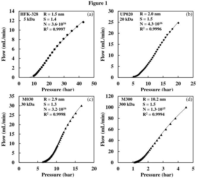
The fitting of R, S and N parameters was carried out for four different membranes with very different MWCOs ranging from 5 to 300 kDa (see Fig. 1). Despite the differences in flow and pressure among membranes, the model fits very well the obtained experimental results with correlation coefficients higher than 0.999 for all membranes. The obtained geometric standard deviations are very similar for most of the membranes (from 1.3 to 1.5). The mean radius increases, as expected, as the MWCO of the membranes increases, following the order HFK-328 (1.5 nm - 5 kDa), UP020 (2.0 nm - 20 kDa), M030 (2.9 nm - 30 kDa) and M300 (10.2 nm - 300 kDa). The total pore number density fluctuates around 4·1016 pore/m2 for the 5, 20 and 30 kDa membranes, but for M300 which has a high mean radius and thus, a lower total pore number density (1.3·1015) is needed to achieve the given flows.

Therefore, a theoretical membrane defined by the three N, R and S parameters can successfully model the flow experimental results of a LLDP analysis for very different membranes.

Figure 1

3 4 5 6 7 8 9 10 11 12 13 14 15 16 17 18 19 20 21 22 23 24 25 26 27 28 29 30 31 32 33 34 35 36 37 38 39 40 41 42 43 44 45 46 47 48 49 50 51 52 53 54 55 56 57 58 59 60

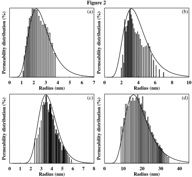
coming from direct application of Grabar-Nikitine algorithm to experimental data, and the fitted ones (solid lines) is remarkable.

Figure 2

4.3. Pore number distribution. Model validation

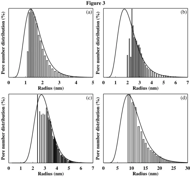
The pore number distribution as a function of the pore radius is represented for the experimental and the modeled membranes to compare the theoretical membrane properties to those of the real one (Fig. 3).

It can be observed that the pore distribution of the HFK-328 theoretical membrane (Fig. 3a) fits very well to the Grabar-Nikitine treated data. For the rest of the membranes (Fig. 3), the pore size distribution fitting is not perfect but satisfactory.

In any case, the agreement between traditionally treated and fitted points is not as good as that obtained for permeability distributions (Fig. 2).This was predictable since permeability distributions come directly from experimental data while pore number ones need a transport model inside the pores to be applied (Hagen-Poiseuille). This was one of the conclusions of the Charmme Network [23] and is nowadays generally accepted

The theoretical distribution accurately matches in the area of higher radii whereas for the lower ones, there is a lack of experimental points. In any case, the agreement for the bigger pores would lead to good enough estimations of MWCO.

4 5 6 7 8 9 10 11 12 13 14 15 16 17 18 19 20 21 22 23 24 25 26 27 28 29 30 31 32 33 34 35 36 37 38 39 40 41 42 43 44 45 46 47 48 49 50 51 52 53 54 55 56 57 58 59 60

software detects non increasing permeabilities. This last procedure (based on a certain tolerance limit introduced by the operator) will prematurely stop the experiment, under certain circumstances, closing abruptly the distribution. Moreover, membranes having very high permeabilities (a usual target for membrane manufacturers) could lead to exhausting the pump reservoir (500 mL) before ending the analysis.

Figure 3

4.4. Permeability and cumulative permeability distribution

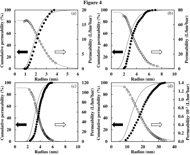
The experimental and modelled permeability cumulative distribution as well as the actual permeability as a function of the pore radius is depicted in Fig. 4. The modelled cumulative distributions of the permeability (closed symbols) do not fit the discretized values as well as it was seen for the differential permeability distribution.

The differences lie in the previously observed lack of experimental data for the lowest radii (high pressures). This implies that the smallest pores are not taken into account to determine their contribution to the global membrane permeability at a given pressure (for a given radius) and so, the permeability cumulative distribution is underestimated when using the experimental results for low radii. This seems more obvious as mean radius (or the MWCO) of the membrane increases, Fig 4d.

3 4 5 6 7 8 9 10 11 12 13 14 15 16 17 18 19 20 21 22 23 24 25 26 27 28 29 30 31 32 33 34 35 36 37 38 39 40 41 42 43 44 45 46 47 48 49 50 51 52 53 54 55 56 57 58 59 60

overall permeability for HFK-328 is much lower to that of the pores around 9.0 nm for the M300 membrane. Therefore, the effect is more pronounced as the MWCO increases.

Nevertheless, the differences found in the individual contribution of each pore size to the overall permeability are not relevant to determine its actual value (Fig. 4, open symbols).

Figure 4

4.5. Advantages of the theoretical model

Once the model was validated, it can be used to improve results in the characterization of any membrane. The most important feature of this model is that it can be applied with a small amount of experimental data, allowing the extrapolation of the membrane performance throughout the LLDP analysis. This is of great importance, especially in quality control areas where saving time and costs are linked and a comprehensive and deep characterization should have done previously. Moreover, this model can also be useful to characterize many membranes in a short period of time, easing the membrane screening for a given process.

4 5 6 7 8 9 10 11 12 13 14 15 16 17 18 19 20 21 22 23 24 25 26 27 28 29 30 31 32 33 34 35 36 37 38 39 40 41 42 43 44 45 46 47 48 49 50 51 52 53 54 55 56 57 58 59 60

accompanied by an error estimation (*) which considers values from the Grabar-Nikitine algorithm as the exact ones. In the case of MWCO, it makes no sense to compare modeled and experimental values as far as we have the nominal values of MWCO given by the membrane manufacturers. So in this case, error (**) accounts for differences between experimental and nominal values.

The information coming from manufacturers was considered reliable, despite they do not specifically state how cut-off was determined [17].

It is also interesting to test if the model still works well when only a small set of the experimental data is used in the fitting. In this sense, what has been done is to fit the developed model to a reduced number of data. In all cases it has been considered a minimum number of six experimental points (except for the last one, ItF, in which only three points were used), but the differences rely in which part of the experimental curve are those data pairs obtained from. Therefore, row In presents the results of the model applied using only the six pairs of flux, pressure data corresponding to the initial part of the experiment (corresponding to lower pressures). Next row (It) shows the fitting results using only six data pairs acquired at the intermediate section of the experiment. In next row (IF), the model was applied using 3 data pairs from the initial part together with the last three pairs. Finally, the last procedure accounts for using one data pair at the beginning of the experiment, another one at intermediate pressure values and last one from the end of the experiment(row ItF).

3 4 5 6 7 8 9 10 11 12 13 14 15 16 17 18 19 20 21 22 23 24 25 26 27 28 29 30 31 32 33 34 35 36 37 38 39 40 41 42 43 44 45 46 47 48 49 50 51 52 53 54 55 56 57 58 59 60

The asymptotic permeability obtained by the model using all the experimental results (tag M) is similar to that experimentally determined for all the membranes, having relative errors lower than 6 %. Differences appear when the fittings are conducted using the results at low (tag In) and intermediate (tag It) pressures (flows), leading to differences around 10-20 %, except in the case of the M300 membrane, for which the fitting was not really possible in these conditions since errors are above 400 %. Nevertheless, when the fittings are conducted either with the data from the beginning (low pressure) and the end (high pressure) of the tests (tag IF) or with three distributed pairs of points (tag ItF) the modelled asymptotic permeability is again similar to the experimental one (tag GN) and to that modelled with all the experimental information (tag M). In fact, differences are lower than 5 % for all the membranes.

4 5 6 7 8 9 10 11 12 13 14 15 16 17 18 19 20 21 22 23 24 25 26 27 28 29 30 31 32 33 34 35 36 37 38 39 40 41 42 43 44 45 46 47 48 49 50 51 52 53 54 55 56 57 58 59 60

number) are relatively small for all the membranes: 1.1 - 1.6 nm, 1.2 - 2.0 nm, 2.2 - 2.6 nm and 8.3 – 11.3 nm for the HFK-328, UP020, M030 and M300 membranes, respectively. And a similar observation can be done for the mean pore radius based on permeability. Therefore, the possibility of using fewer experimental data to estimate the mean pore radius of the membranes using the proposed model is feasible.

The estimation of the MWCO leads to different conclusions depending on the membranes. The estimation of the HFK-328 and M300 membrane MWCOs is more accurate using the model (tag M) than using the Grabar-Nikitine algorithm results (GN), while for the UP020 and M030 membranes the model only allows an estimate of the order of magnitude of MWCO.

One of the shortcomings of applying this model to small amounts of experimental data is that the results could be incoherent. For instance, using the procedures (In) and (It) for very open UF membranes, such as the M300 membrane, the results are not successful because there is a lack of information in the high pressure area which is associated to the asymptotic permeability. Therefore, in these cases, a careful analysis of the results should be carried out, leading the LLDP experiment to include more high pressure points to avoid such errors.

Table 2

5. Conclusions

3 4 5 6 7 8 9 10 11 12 13 14 15 16 17 18 19 20 21 22 23 24 25 26 27 28 29 30 31 32 33 34 35 36 37 38 39 40 41 42 43 44 45 46 47 48 49 50 51 52 53 54 55 56 57 58 59 60

Comparing the expected behavior of the model with the actual results, the log-normally shaped distribution is a reasonable choice.

The accuracy of the fitting approach has been tested with several polymeric membranes having an expected large range of pores, according to the nominal MWCO values. Results of the fitting are reasonably good and in accordance with most of the parameters arising from traditional LLDP analysis.

The use of partial data does not guarantee good results or show a clear trend in data analysis, in any case this partial analysis do not lead to worse results.

It must not be forgotten that a good fitting is only possible if good data is collected. Whatever is the procedure for measuring or fitting data, LLDP experiments are not and they will never be so easy to perform as GLDP ones, where only 5 min are enough to get a good pore size distribution.

On the contrary LLDP experiments need longer time (never less than 1 h), so any approach aimed to reduce the number of experimental points, such as that considered in this work, requires a reliable data fitting for a possible extensive or commercial use of the technique.

Acknowledgements

Authors gratefully acknowledge the financial support given by: Junta de Castilla y León (Project VA248U13), Spanish Ministry of Science and Innovation (projects MAT2011-25513 and CTQ2012-31076) and the Spanish Ministry of Education, Culture and Sports via a collaboration scholarship and a FPU grant (AP2010-3549).

Nomenclature

4 5 6 7 8 9 10 11 12 13 14 15 16 17 18 19 20 21 22 23 24 25 26 27 28 29 30 31 32 33 34 35 36 37 38 39 40 41 42 43 44 45 46 47 48 49 50 51 52 53 54 55 56 57 58 59 60

D∞: Diffusion coefficient of the dextran at infinite dilution in water (m2/s)

ek: Difference between the experimental and the modelled membrane flow (m3/s) F: Membrane flux (m3/m2s)

fL(r): Probability distribution function for the permeability from pores of radius r (m-1) fn(r): Probability distribution function for the number of pores of radius r (m-1)

J: Membrane flow (m3/s) l: Pore length

MWCO: Molecular weight cut-off (Da) n(r): Pore number distribution (pore/m3) N: Total pore number density (pore/m2)

NAB: Pore number density with radii between rA and rB (pore/m2) ΔP: Transmembrane pressure (Pa)

R: Geometric mean radius or location parameter (m) r: radius (m)

<r>number: Mean radius based on the pore number distribution (m) <r>perm: Mean radius based on the permeability distribution (m) S: Geometric standard deviation or scale parameter (dimensionless)

Greek letters

η: Viscosity (Pa·s)

3 4 5 6 7 8 9 10 11 12 13 14 15 16 17 18 19 20 21 22 23 24 25 26 27 28 29 30 31 32 33 34 35 36 37 38 39 40 41 42 43 44 45 46 47 48 49 50 51 52 53 54 55 56 57 58 59 60

References

[1] D. Li, M.W. Frey, Y.L. Joo, Characterization of nanofibrous membranes with capillary flow porometry, Journal of Membrane Science, 286 (2006) 104-114.

[2] S. S. Manickam, J.R. McCutcheon, Characterization of polymeric nonwovens using porosimetry, porometry and X-ray computed tomography, Journal of Membrane Science, 407–408 (2012) 108-115.

[3] S. Munari, A. Bottino, G.C. Roda, G. Capannelli, Preparation of ultrafiltration membranes. State of the art, Desalination, 77 (1990) 85-100.

[4] P. Abaticchio, A. Bottino, G.C. Roda, G. Capannelli, S. Munari, Characterization of ultrafiltration polymeric membranes, Desalination, 78 (1990) 235-255.

[5] J.I. Calvo, A. Bottino, P. Prádanos, L. Palacio, A. Hernández, Porosity, in: E.M.V. Hoek, V.V. Tarabara (Eds.) Encyclopedia of Membrane Science and Technology, John Wiley and Sons, Hoboken, NJ (USA), 2014.

[6] A. Hernández, J.I. Calvo, P. Prádanos, F. Tejerina, Pore size distributions in microporous membranes. A critical analysis of the bubble point extended method, Journal of Membrane Science, 112 (1996) 1-12.

[7] K.R. Morison, A comparison of liquid–liquid porosimetry equations for evaluation of pore size distribution, Journal of Membrane Science, 325 (2008) 301-310.

[8] T.N. Shah, H.C. Foley, A.L. Zydney, Development and characterization of nanoporous carbon membranes for protein ultrafiltration, Journal of Membrane Science, 295 (2007) 40-49.

4 5 6 7 8 9 10 11 12 13 14 15 16 17 18 19 20 21 22 23 24 25 26 27 28 29 30 31 32 33 34 35 36 37 38 39 40 41 42 43 44 45 46 47 48 49 50 51 52 53 54 55 56 57 58 59 60

[10] P. Aimar, M. Meireles, V. Sanchez, A contribution to the translation of retention curves into pore size distributions for sieving membranes, Journal of Membrane Science, 54 (1990) 321-338.

[11] K.D. Knierim, M. Waldman, E.A. Mason, Bounds on solute flux and pore-size distributions for non-sieving membranes, Journal of Membrane Science, 17 (1984) 173-203.

[12] K.D. Knierim, E.A. Mason, Heteroporous sieving membranes: Rigorous bounds on pore-size distributions and sieving curves, Journal of Membrane Science, 42 (1989) 87-107. [13] A.L. Zydney, P. Aimar, M. Meireles, J.M. Pimbley, G. Belfort, Use of the log-normal probability density function to analyze membrane pore size distributions: functional forms and discrepancies, Journal of Membrane Science, 91 (1994) 293-298.

[14] P. Grabar, S. Nikitine, Sur le diamètre des pores des membranes en collodion utilisées en ultrafiltration, Journal of Chemical Physics, 33 (1936) 721-741.

[15] F. Erbe, The determination of pore distributions according to sizes in filters and ultrafilters, Kolloid-Z, 63 (1933) 277-285.

[16] S. Derjani-Bayeh, V.G.J. Rodgers, Sieving variations due to the choice in pore size distribution model, Journal of Membrane Science, 209 (2002) 1-17.

[17] J.I. Calvo, R.I. Peinador, P. Prádanos, L. Palacio, A. Bottino, G. Capannelli, A. Hernández, Liquid–liquid displacement porometry to estimate the molecular weight cut-off of ultrafiltration membranes, Desalination, 268 (2011) 174-181.

3 4 5 6 7 8 9 10 11 12 13 14 15 16 17 18 19 20 21 22 23 24 25 26 27 28 29 30 31 32 33 34 35 36 37 38 39 40 41 42 43 44 45 46 47 48 49 50 51 52 53 54 55 56 57 58 59 60

[19] J.M. Sanz, R. Peinador, J.I. Calvo, A. Hernández, A. Bottino, G. Capannelli, Characterization of UF membranes by liquid–liquid displacement porosimetry, Desalination, 245 (2009) 546-553.

[20] M.C. Almécija, J.E. Zapata, A. Martinez-Ferez, A. Guadix, A. Hernández, J.I. Calvo, E.M. Guadix, Analysis of cleaning protocols in ceramic membranes by liquid–liquid displacement porosimetry, Desalination, 245 (2009) 541-545.

[21] J.I. Calvo, A. Bottino, G. Capannelli, A. Hernández, Pore size distribution of ceramic UF membranes by liquid–liquid displacement porosimetry, Journal of Membrane Science, 310 (2008) 531-538.

[22] J.I. Calvo, A. Bottino, G. Capannelli, A. Hernández, Comparison of liquid–liquid displacement porosimetry and scanning electron microscopy image analysis to characterise ultrafiltration track-etched membranes, Journal of Membrane Science, 239 (2004) 189-197. [23] CHARMME Network “Harmonization of characterization methodologies for porous membranes”, EC Contract SMT4-CT 98-7518. Web page:

4 5 6 7 8 9 10 11 12 13 14 15 16 17 18 19 20 21 22 23 24 25 26 27 28 29 30 31 32 33 34 35 36 37 38 39 40 41 42 43 44 45 46 47 48 49 50 51 52 53 54 55 56 57 58 59 60

3 4 5 6 7 8 9 10 11 12 13 14 15 16 17 18 19 20 21 22 23 24 25 26 27 28 29 30 31 32 33 34 35 36 37 38 39 40 41 42 43 44 45 46 47 48 49 50 51 52 53 54 55 56 57 58 59 60 Figure 1

Fig. 1. Experimental results obtained through LLDP (symbols) and fitted model (solid line) for HFK-328 (a), UP020 (b), M030 (c), and M300 (d) membranes.

0 2 4 6 8 10 12 14

0 10 20 30 40 50

F low ( m L /m in ) Pressure (bar) HFK-328 5 kDa

R = 1.5 nm S = 1.4 N = 3.6·1016 R2_{= 0.9997}

0 5 10 15 20 25 30

0 5 10 15 20 25

F low ( m L /m in ) Pressure (bar) UP020 20 kDa

R = 2.0 nm S = 1.5 N = 4.3·1016 R2_{= 0.9996}

0 5 10 15 20 25 30 35

0 5 10 15 20

F low ( m L /m in ) Pressure (bar) M030 30 kDa

R = 2.9 nm S = 1.3 N = 3.2·1016

R2_{= 0.9998}

0 20 40 60 80 100 120

0 1 2 3 4 5

F low ( m L /m in ) Pressure (bar) M300 300 kDa

R = 10.2 nm S = 1.5 N = 1.3·1015

R2_{= 0.9994}

(a) (b)

4 5 6 7 8 9 10 11 12 13 14 15 16 17 18 19 20 21 22 23 24 25 26 27 28 29 30 31 32 33 34 35 36 37 38 39 40 41 42 43 44 45 46 47 48 49 50 51 52 53 54 55 56 57 58 59 60

Figure 2

Fig. 2. Experimental (bars) and modeled (solid line) permeability distribution of HFK-328 (a), UP020 (b), M030 (c) and M300 (d) membranes.

Radius (nm)

0 10 20 30 40

P

erm

ea

bil

it

y

dis

tri

but

io

n (

%

)

Radius (nm)

0 1 2 3 4 5 6 7 8

P

erm

ea

bil

it

y

dis

tri

but

io

n (

%

)

Radius (nm)

0 2 4 6 8 10

P

erm

ea

bil

it

y

dis

tri

but

io

n (

%

)

Radius (nm)

0 1 2 3 4 5 6 7

P

erm

ea

bil

it

y

dis

tri

but

io

n (

%

) (a) (b)

3 4 5 6 7 8 9 10 11 12 13 14 15 16 17 18 19 20 21 22 23 24 25 26 27 28 29 30 31 32 33 34 35 36 37 38 39 40 41 42 43 44 45 46 47 48 49 50 51 52 53 54 55 56 57 58 59 60

Figure 3

Fig. 3. Experimental (bars) and modelled (solid line) pore number distribution of HFK-328 (a), UP020 (b), M030 (c) and M300 (d) membranes.

Radius (nm)

0 1 2 3 4 5 6 7

P

ore n

umber

dist

ribut

io

n

(%

)

Radius (nm)

0 5 10 15 20 25 30

P

ore n

umber

dist

ribut

io

n

(%

)

Radius (nm)

0 1 2 3 4 5

P

ore n

umber

dist

ribut

io

n

(%

)

Radius (nm)

0 1 2 3 4 5 6 7

P

ore n

umber

dist

ribut

io

n

(%

)

(a) (b)

4 5 6 7 8 9 10 11 12 13 14 15 16 17 18 19 20 21 22 23 24 25 26 27 28 29 30 31 32 33 34 35 36 37 38 39 40 41 42 43 44 45 46 47 48 49 50 51 52 53 54 55 56 57 58 59 60 Figure 4

Fig. 4. Experimental (closed symbols) and modelled (solid line) cumulative permeability distribution as well as experimental (open symbols) and modelled (dotted line) permeability as function of pore size for the HFK-328 (a), UP020 (b), M030 (c) and M300 (d) membranes. 0 20 40 60 80 100 120 0 20 40 60 80 100

0 2 4 6 8 10

P er m eab il ity (L/h m 2b ar ) C u m u lati ve p er m eab il ity (% ) Radius (nm) 0.0 0.2 0.4 0.6 0.8 1.0 1.2 1.4 0 20 40 60 80 100

0 10 20 30 40

P er m eabi lity· 10 -3 (L/ hm 2bar) C u m u lati ve p er m eab il ity (% ) Radius (nm) 0 5 10 15 20 0 20 40 60 80 100

0 1 2 3 4 5 6

P er m eab il ity (L/h m 2b ar ) C u m u lati ve p er m eab il ity (% ) Radius (nm) 0 20 40 60 80 0 20 40 60 80 100

0 2 4 6 8 10

3 4 5 6 7 8 9 10 11 12 13 14 15 16 17 18 19 20 21 22 23 24 25 26 27 28 29 30 31 32 33 34 35 36 37 38 39 40 41 42 43 44 45 46 47 48 49 50 51 52 53 54 55 56 57 58 59 60

4 5 6 7 8 9 10 11 12 13 14 15 16 17 18 19 20 21 22 23 24 25 26 27 28 29 30 31 32 33 34 35 36 37 38 39 40 41 42 43 44 45 46 47 48 49 50 51 52 53 54 55 56 57 58 59 60

Table 1: Membrane properties according to manufacturers.

Membrane Material Manufacturer MWCO (kDa)

HFK-328

Polyethersulfone Koch 5

UP020 Nadir 20

Minitan M030

Polysulfone Millipore 30

3 4 5 6 7 8 9 10 11 12 13 14 15 16 17 18 19 20 21 22 23 24 25 26 27 28 29 30 31 32 33 34 35 36 37 38 39 40 41 42 43 44

Membr. Math.

proced.

Asymptotic permeability

(L/hm2bar)

Relative error (%)

(* - ***)

Mean radius - Pore number

(nm)

Relative error (%)

(* - ***)

Mean radius - Permeability

(nm)

Relative error (%)

(* - ***)

MWCO (kDa)

Relative error (%)

(**)

R

(nm) S N

HFK-328

GN 16.5 - 1.7 - 2.3 - 6.9 38 - -

-M 16.5 1* 1.2 27* 2.1 9* 4.7 6 1.5 1.44 3.7·1016

In 17.0 3*** 1.3 8*** 2.1 3*** 5.3 7 1.6 1.42 3.3·1016

It 17.0 3*** 1.1 13*** 2.0 5*** 3.7 26 1.3 1.48 5.0·1016

IF 16.3 1*** 1.6 28*** 2.3 11*** 7.2 43 1.8 1.37 2.2·1016

ItF 16.1 2*** 1.2 1*** 2.1 1*** 4.8 3 1.5 1.44 3.5·1016

UP020

GN 72 - 2.8 - 3.5 - 18 8 - -

-M 77 6* 1.6 42* 3.0 17* 9 56 2.0 1.48 4.3·1016

In 87 12*** 1.2 28*** 2.5 15*** 5 75 1.6 1.55 1.0·1017

It 68 12*** 1.9 17*** 3.2 9*** 12 41 2.3 1.44 2.7·1016

IF 74 4*** 2.0 24*** 3.3 11*** 13 35 2.4 1.42 2.6·1016

ItF 76 1*** 1.5 9*** 2.9 2*** 8 62 1.9 1.51 4.9·1016

M030

GN 106 - 3.4 - 3.9 - 27 9 - -

-M 110 3* 2.6 22* 3.3 14* 19 38 2.9 1.27 3.2·1016

In 116 6*** 2.2 15*** 3.0 9*** 14 53 2.5 1.32 5.0·1016

It 123 13*** 2.3 13*** 3.1 7*** 15 51 2.6 1.32 5.0·1016

IF 110 1*** 2.5 5*** 3.3 2*** 17 43 2.8 1.29 3.5·1016

ItF 112 2*** 2.4 8*** 3.2 4*** 16 46 2.7 1.30 3.9·1016

M300

GN 1302 - 13.2 - 19.6 - 629 110 - -

-M 1322 2* 8.3 37* 14.4 27* 261 13 10.2 1.45 1.3·1015

In 10365 700*** 5.5 34*** 9.7 33*** 111 63 6.8 1.46 5.0·1016

It 6160 400*** 4.5 46*** 9.0 38*** 78 74 5.8 1.52 4.3·1016

IF 1334 1*** 8.6 5*** 14.0 3*** 271 10 10.3 1.41 1.4·1015

ItF 1308 1*** 11.3 37*** 16.1 12*** 430 43 12.9 1.35 7.4·1014

GN: Experimental results

M: Fitted with all experimental data In: Fitted with the first six pairs of data