An empirical application of stochastic volatility models to Latin-American stock returns using GH skew student's t-distribution

PONTIFICIA UNIVERSIDAD CATÓLICA DEL PERÚ

ESCUELA DE POSGRADO

“An Empirical Application of Stochastic Volatility Models to

Latin-American Stock Returns using GH Skew Student´s

t

Tesis para optar el grado de Magíster en Estadística

AUTOR

Patricia Lengua Lafosse

ASESOR

Cristian Bayes

JURADO

Luis Valdivieso

Oscar Millones

An Empirical Application of Stochastic Volatility Models to

Latin-American Stock Returns using

GH

Skew Student’s

t

-Distribution

Patricia Lengua Lafossey

Ponti…cia Universidad Católica del Perú Thesis Advisor: Cristian Bayes z Ponti…cia Universidad Católica del Perú

March 12, 2015

Abstract

This paper represents empirical studies of stochastic volatility (SV) models for daily stocks returns data of a set of Latin American countries (Argentina, Brazil, Chile, Mexico and Peru) for the sample period 1996:01-2013:12. We estimate SV models incorporating both leverage e¤ects and skewed heavy-tailed disturbances taking into account the GH Skew Student’s t -distribution using the Bayesian estimation method proposed byNakajima and Omori(2012). A model comparison between the competing SV models with symmetric Student´st-disturbances is provided using the log marginal likelihoods in the empirical study. A prior sensitivity analysis is also provided. The results suggest that there are leverage e¤ects in all indices considered but there is not enough evidence for Peru, and skewed heavy-tailed disturbances is con…rmed only for Argentina, symmetric heavy-tailed disturbances for Mexico, Brazil and Chile, and symmetric Normal disturbances for Peru. Furthermore, we …nd that theGH Skew Student’st-disturbance distribution in the SV model is successful in describing the distribution of the daily stock return data for Peru, Argentina and Brazil over the traditional symmetric Student´s t-disturbance distribution.

JEL Classi…cation: C11, C58.

KeyWords:Stochastic Volatility, Generalized Hyperbolic Skew Student’st-Distribution, Bayesian Estimation, Markov Chain Monte Carlo, Stock Returns, Latin American Stock Markets.

We are grateful to Gabriel Rodríguez for helpful comments and suggestions.

1 Introduction

Returns from …nancial market variables such as stock and exchange rate are characterized by some empirical properties which are generally presented in …nancial time series. There are three important stylized facts or properties that are found in almost all set of daily returns: i) returns are not normally distributed; instead, the characteristics of the return distributions are excess of kurtosis (leptokurtic) and some degree of skewness compared with the Normal distribution1, ii) there is almost no correlation between daily returns at di¤erent lags and iii) functions of returns can have substantial autocorrelations. For example, the autocorrelation of both absolute returns and squared returns are positive for many lags and statistically signi…cative (Taylor,2005). These properties are explained in most cases by the presence of time-varying volatility and volatility clustering over time.

Modelling time-varying volatility has been widely used in the literature of …nancial time series, as the demand for volatility forecasts has increase to assess the …nancial risk. Two approaches that have proven useful are the autoregressive conditional heteroskedasticity (ARCH) family, including ARCH model developed by Engle (1982) and generalized ARCH (GARCH) model of Bollerslev

(1986), and the stochastic volatility (SV) model, …rst introduced by Taylor (1982), then Taylor

(1986) was the …rst lengthy published treatment of the problem of volatility modelling in …nance. For extensive reviews, see Bollerslev et al. (1994) and Engle (1995) for the ARCH family models andShephard (2005) provide a comprehensive explanation of the SV models. Both approaches try to model and reproduce the principal properties of the asset returns; however, the di¤erence is that ARCH models explicitly model and specify a process for the conditional variance of returns given past returns observed; while the SV models involve specifying a stochastic process for the volatility and this is modelled as an unobserved variable.

Departures from normality have originated propositions of other distributions in order to capture heavy-tailedness of the asset return distribution in the SV class of models. Heavy-tailed distur-bances are often incorporated using distributions such as Student’st-distribution (see, for example,

Harvey et al. (1994), Liesenfeld and Jung (2000), Chib et al. (2002), Berg et al. (2004), Jacquier et al.(2004),Omori et al.(2007),Asai(2008),Choy et al.(2008),Nakajima and Omori(2009),Asai and McAleer (2011), Wang et al. (2011), Nakajima (2012) and Delatola and Gri¢n (2013)), the Normal Inverse Gaussian distribution (NIG, see Barndor¤-Nielsen (1997) and Andersson (2001)), the Generalized Error Distribution (GED, seeLiesenfeld and Jung(2000)), the Generalized-t distri-bution (GT, seeWang(2012) and Wang et al. (2013)), a class of mixtures of Normal distributions (Abanto-Valle et al., 2010; Asai, 2009) and, to allow simultaneously treatment of skewness and heavy tails in the conditional distribution of returns, the Skew-GED distribution (Cappuccio et al.,

2004,2006), the Extended Generalized Inverse Gaussian (EGIG, seeSilva et al. (2006)), the Skew Student’st-distribution (Tsiotas,2012;Abanto-Valle et al.,2013) and the Generalized Hyperbolic (GH) Skew Student’st-distribution (Nakajima and Omori,2012;Trojan,2013)2.

Another characteristic of the return distribution for …nancial variables is the asymmetric

re-1_{In most cases, it is a negative skewness and it can be viewed as the case where negative returns of a given}

magnitude are more likely than positive ones of the same magnitude. Regarding excess of kurtosis, it can be viewed as the case where extreme values are more likely than would be dictated by a Normal distribution.

2_{In fact, the GT-family nests a number of well-known distributions including Normal, Student-t, Laplace and}

sponse of volatility known as the “leverage e¤ect”: negative past innovations on asset returns tend to increase the current volatility. First noted byBlack(1976) and studied byNelson(1991) andYu

(2005), leverage e¤ect refers to the tendency for changes in asset prices to be negatively correlated with changes in asset volatility. Leverage e¤ect is an important stylized fact of especially stock return indices and has motivated consideration of asymmetric extensions of the basic SV model.

Time-varying volatility for …nancial variables of developed economies have been studied ex-tensively; however, empirical studies of the Latin American stock market indices so far are very scarce. The volatility characteristics of the …nancial markets in Latin America are far from being thoroughly analyzed despite their growth in recent years. The main aim of this paper is to estimate SV models incorporating both leverage e¤ects and skewed heavy-tailed disturbances taking into ac-count theGH Skew Student’st-distribution for the Latin American stock market indices using the Bayesian estimation method proposed by Nakajima and Omori (2012). The GH skew Student’s t-distribution includes Normal and Student’s t-distributions as special cases. Therefore, the SV model using the GH Skew Student’s t-distribution (SVSKt model) can take a ‡exible form to …t the returns and volatility characteristics because the SVSKt model is able to model substantially skewed and heavy tailed data and includes the SV model with Normal disturbances (SV-Normal) and the SV model with symmetric Student’s t-disturbances (SVt). We apply the SVSKt model to daily returns of …ve Latin American stock market indices: Peru, Argentina, Mexico, Chile and Brazil. We also include the U.S. S&P500 returns in order to perdorm some comparisons.

The GH Skew Student’s t-distribution has been studied by Aas and Ha¤ (2006) and brie‡y mentioned by Prause(1999) and Jones and Faddy (2003). It belongs to the class of GH distribu-tions introduced byBarndor¤-Nielsen(1977) and extensively discussed byPrause(1999). TheGH

distribution is a Normal variance-mean mixture and possesses a number of attractive properties: it is closed under conditioning, marginalization, and a¢ne transformations, ii) GH distribution can be both symmetric and skew, and its tails are generally semiheavy and iii) GH distribu-tion embraces many special cases including Normal, Hyperbolic, Normal Inverse Gaussian (NIG), Variance-Gamma, Student-tand skew Student’st-distributions (Aas and Ha¤,2006;Nakajima and Omori, 2012). However, estimation and identi…cation of its parameters can be di¢cult in general due to the ‡atness of the likelihood function, some parameters are hard to separate and the likeli-hood function may have several local maxima (Prause,1999;Aas and Ha¤,2006;Deschamps,2012). NeverthelessAas and Ha¤ (2006) noted that the GH Skew Student’st-distribution is analytically tractable and it may considerably alleviate the identi…cation problem mentioned above. Another advantage is that the GH Skew Student’s t-distribution exhibit unequal thickness in both tails, unlike to other skewed extensions of the Student-tdistribution. This distribution has the property that one tail has polynomial and the other exponential behavior and this o¤ers more ‡exibility3.

A main di¢culty of the SV framework is the parameter estimation because no explicit expression for the likelihood function of SV model is directly available due to the fact that the variance is an unobserved component. It is possible to compute the likelihood function but this requires the use of simulation techniques, like simulated maximum likelihood, method of simulated moments or Markov Chain Monte Carlo (MCMC) techniques. For an overview of estimation methods of SV models, see Shephard (1996, 2005); Ghysels et al. (1996); Broto and Ruiz (2004). Simulation

3_{Several articles have studied di¤erent skew t-type distributions where distributions have two tails behaving as}

techniques require a computational burden since we need to repeat the …ltering procedure many times to evaluate the likelihood function for each set of parameters until it reaches the maximum (Nakajima,2012). Computer-intesive methods are thus needed even for the simplest version of the model4. In addition,Nakajima and Omori(2012) noted that theGH Skew Student’st-distribution is di¢cult to implement in the SV context due to the large numbers of latent volatility variables. To overcome this di¢culty,Nakajima and Omori(2012) have proposed a Bayesian estimation method using the MCMC algorithm for a precise and e¢cient estimation of the SV model including both leverage e¤ects and skewed heavy-tailed disturbances using theGH Skew Student’st-distribution. The key point to implement an e¢cient MCMC algorithm in the SVSKt model is to express the

GH Skew Student’s t-distribution of the disturbance as a Normal variance-mean mixture of the Generalized Inverse Gaussian (GIG), speci…cally the Inverse Gamma (IG) distribution as a mixing distribution among the class ofGIG distributions to nest and extend various existing SV models.

The paper is organized as follows. In Section 2, we describe a basic SV-Normal model and introduce the GH Skew Student’s t-distribution in the SV context (SVSKt model). In addition, we describe the Bayesian estimation method using the MCMC algorithm proposed by Nakajima and Omori(2012). Section 3 presents empirical results based on …ve Latin American stock market indices: Peru, Argentina, Mexico, Chile and Brazil, where the SVSKt model is applied to daily return data using the estimation method proposed by Nakajima and Omori (2012) and the com-peting SVt models are compared. In order to compare results, the SVSKt is also applied to US S&P500 daily return data. A prior sensitivity analysis is also provided in this Section. Conclusions are presented in Section 4. In the Appendix, we present the properties of theGH Skew Student’s t-distribution, the MCMC sampling procedure in detail and the Multi-move sampler for the SVSKt model used by Nakajima and Omori (2012).

2 Bayesian Inference for the SV Model with Leverage and Skewed Heavy-Tailed Disturbances using the GH _{Skew Student’s t-Distribution}

2.1 A Basic SV Model

The SV models assume that the volatility of stock returns has been generated under a latent stochastic process. The basic discrete-time SV model with Normal disturbances can be written as

yt = exp(ht=2) t; t= 1; : : : ; n; (1)

ht+1 = + (ht ) + t; t= 0; : : : ; n 1; (2)

t N(0;1); (3)

t N(0; 2); (4)

where yt is the asset return and ht is the unobserved logarithm of the volatility. The volatility

process is commonly assumed to follow a stationary AR(1) process by imposing that the persistence parameter satis…es the condition _{j j} < 1; this imply that the log-volatility process is stationary and the initial value, h1, is assumed to follow a stationary distribution by setting h0 = and

0 N(0; 2=(1 2)). Finally, t and t are uncorrelated Normal distributed disturbances. 4_{Despite the computational costs that these techniques involving, increasing computer power and the further}

There are characteristics of the return distribution for …nancial variables that the basic SV model with Normal disturbances does not capture such as excess of kurtosis and heavy-tailedness, skewness and the leverage e¤ects. The excess of kurtosis and skewness of the asset return distribution justify the introduction of skewed heavy-tailed disturbances such as theGH Skew Student’st-distribution. On the side of the leverage e¤ects, the basic SV model does not allow that the volatility reacts with positive or negative movements in returns. These leverage e¤ects can be incorporated in the SV model assuming that there is any association between the return shocks ( t) and volatility shocks

( _t).

2.2 A SV Model with Leverage and Skewed Heavy-Tailed Disturbances

According to Nakajima and Omori (2012), the SV model with leverage e¤ects can be written as:

yt = exp(ht=2) t; t= 1; : : : ; n; (5)

ht+1 = + (ht ) + t; t= 0; : : : ; n 1; (6) t

t N(0; ); with =

h₁ 2

i

: (7)

This model is similar to previous basic SV model, but now we allow that t and t are correlated

disturbances where the parameter measures the correlations between tand t. We have volatility

asymmetry if ₆= 0 and speci…cally, when <0, this indicates a leverage e¤ect: a negative return today will increase volatility tomorrow, and when = 0, there is not this type of e¤ects (Yu,2005). Regarding the SV model incorporating both leverage e¤ects and skewed heavy-tailed distur-bances using the GH Skew Student’s t-distribution, skewed heavy tails in the return distribution is incorporated into the SV model by replacing the Normal disturbance t in (5) by a disturbance

from a GH Skew Student’s t-distribution, denoted by !t. This GH Skew Student’s t-distribution

is a limiting case of the more general class of the GH distribution. Following Prause (1999) and

Aas and Ha¤ (2006), the probability density function of aGH random variable!_t is given by:

fGH(! ; ; ; ; !; ) =

( 2 2) =2K 1=2 q

2_{+ (!}

!)2 exp ( (! !))

p

2 1=2 _K p 2 2 q 2_{+ (x}

!)2

1=2 ; (8)

whereKj is the modi…ed Bessel function of the third kind of orderjand the parameters must ful…ll

certain conditions; for more details see Appendix A. The GH distribution may be represented as a Normal variance-mean mixture with the Generalized Inverse Gaussian (GIG) distribution as a mixing distribution. This means that the GH variable!_t can be represented as:

!_t = _!+ z_t +pz_{t t}; t N(0;1); zt GIG( ; ; ); (9)

with t and zt independent and = p

2 2_{. The GH Skew Student’s t-distribution is the}

fGHskewt(!; ; ; !; ) =

212 j j

v+1 2 K_v+1

2

r

2 2_{+ (!}

!)2 exp ( (! !))

(v₂)p

q

2_{+ (!}

!)2

v+1 2

; ₆= 0;

(10) and

fGHskewt(!; ; ; !) =

(v+1₂ )

p ₍v 2)

"

1 +(! !)

2

2

# (v+1)=2

; = 0: (11)

where (:) is the gamma function. The density fGHskewt(!; ; ; !) in (11) is known as the

non-central Student’st-distribution with degrees of freedom.

As observed in the literature, estimation and identi…cation of GH distribution parameters can be di¢cult in general (Prause, 1999;Aas and Ha¤,2006; Deschamps, 2012) even for a GH Skew Student’s t-distribution with = =2 ( >0) and = 0 (Nakajima and Omori,2012). In order to overcome these di¢culties, Nakajima and Omori (2012) make the additional assumption that =p and, show that their proposed parameterization is appropriate for the SV model with the

GH Skew Student’s t-distribution because it allows a parsimonious representation that is more amenable to estimation and leads an e¢cient MCMC sampling. This additional assumption yields z_t =zt GIG( =2;p ;0), or equivalently IG( =2; =2) where IG denotes the Inverse Gamma

distribution. Therefore, the GH Skew Student’st-disturbance, !t, can be express in the form of

the normal variance-mean mixture as:

!t= !+ zt+pzt t; t N(0;1); zt IG( =2; =2); (12)

where _! and are the location and skew parameters, respectively and the IG distribution is the mixing distribution among the class ofGIG distributions. Nakajima and Omori(2012) argue that the structure of (12) leans itself well to the construction of a MCMC algorithm in the Bayesian inference context. To allowE(!t) = 0, it is assumed that ! = z, where z E(zt) = =( 2).

The variance of!t is only …nite when >4, as opposed to the symmetric Student’st-distribution

which only requires >2, because of that an additional constraint is imposed, >4, in order to ensure existence of the second moment of!t.

Figure 1. Densities of the GH Skew Student’st-distribution. Parameter varying using = 0(symmetric

t), 2 and 4 with = 10…xed (top); and parameter varying using = 5,10 and15with = 2

…xed (bottom).

Taking into account the above issues, the SV model incorporating both leverage e¤ects and skewed heavy-tailed disturbances using theGH Skew Student’st-distribution (SVSKt model) can be written as:

yt = exp(ht=2)f (zt z) +pzt tg; t= 1; : : : ; n; (13)

ht+1 = + (ht ) + t; t= 0; : : : ; n 1; (14)

zt IG( =2; =2); (15)

t

t N(0; ); with =

h₁ 2

i

: (16)

The degree of freedom > 4 is unknown to be estimated. The SVSKt model includes the SV model with Normal disturbances (SV-Normal) when = 0 and zt 1 for allt and the SV model

with symmetric Student’st-disturbances (SVt) when = 0.

2.3 Bayesian Estimation of the SVSKt Model

estimation of SV models within the Bayesian context and a brie‡y discussion about the steps of the MCMC algorithm ofNakajima and Omori (2012).

Estimation of SV models consists of two stages: estimation of the set of parameters of the model, and estimation of the unobserved volatility time series. Techniques based on MCMC algorithms o¤er a framework both for estimating the parameters of the SV models and for assessing the latent volatilities. These methods have had a widespread in‡uence on the theory and practice of Bayesian inference that are based on the posterior distributions of parameters given the observed data using the Bayes Theorem, where ( _j y) _f(y j ) ( ) is the the posterior distribution of

parameters conditional on the data y, is the vector that contains all parameters of the model, f(y_j )is the likelihood function, and ( ) are the priors which are beliefs about the distributions of the parameters. The idea behind the MCMC algorithms is to produce random variables from a given multivariate density (the posterior density in Bayesian applications) by repeatedly sampling a Markov chain whose invariant distribution is the target density of interest (Kim et al., 1998). There are typically many di¤erent ways of constructing a Markov chain with this property; but a key point is to isolate those that are simulation-e¢cient in the context of SV models, therefore the design of the MCMC algorithm is important for the speed of convergence of the chains.

In the SV context, the likelihood function to be maximized is given by:

f(y_j ) =

Z

f(y_jh; )f(h_j )dh: (17)

where is the vector that contains all parameters of the SV model. Jacquier et al. (1994) argue that the likelihood function has no analytical representation and is intractable. This fact precludes the direct analysis of the posterior density ( _j y) by MCMC methods. This problem can be overcome by focusing instead on the density ( ; h_jy);where h = (h1; : : : ; hn) is the vector ofn

latent log-volatilities (Kim et al.,1998). The MCMC procedures can be developed to sample this density without computation of the likelihood functionf(y_j ). These draws can be used to make inferences by appealing to suitable ergodic Theorems for Markov chains. For example, posterior moments and marginal densities can be estimated by averaging the relevant function of interest over the sampled random variables. The posterior mean of is estimated by the sample mean of the simulated values.

Several approaches of MCMC algorithms have been suggested for the estimation of the SV model within the Bayesian context. Jacquier et al. (1994) use the single-move Gibbs sampling within the Metropolis–Hastings algorithm to sample from the log-volatilities h = (h1; : : : ; hn).

This algorithm consists of generating sample of one state, ht, at a time given others, hk (k 6=t).

Some researchers have argued that when parameters are correlated, the single-move procedure results in a slower speed of convergence of the Markov chain. Kim et al. (1998) developed the mixture sampler that approximates the distribution of log-squared returns by mixture of Normal distributions, allowing jointly drawing on the components of the whole vector of log-volatilities. Another approach, developed byShephard and Pitt(1997) andWatanabe and Omori(2004) in the context of state space modeling, uses the multi-move sampler for generating the log-volatility in the SV model updating several variables at a time. This algorithm can produce e¢cient samples from the target conditional posterior distribution by dividing the process of h = (h1; : : : ; hn) into

than the single-move sampler that generate sample of one state, ht, at a time given others, hk

(k₆=t) (Nakajima,2012).

The Bayesian estimation method proposed by Nakajima and Omori (2012) for the SVSKt model extends the method developed by Omori and Watanabe (2008) for sampling h using the multi-move sampler. They noted that the key point to implement an e¢cient MCMC algorithm in the SVSKt model is to express theGH Skew Student’st-distribution of the disturbance as a Normal variance-mean mixture of the GIG, as stated in (12), speci…cally the IG distribution as a mixing distribution among the class of GIG distributions. They consider the variable zt, following the

mixing distribution, as a latent variable. The conditional posterior distribution of each parameter is reduced to a much more tractable form conditional on zt than when the model is considered in

the direct likelihood form of theGH Skew Student’st-distribution5_{. This treatment allows to draw}

sample from the conditional posterior distribution ofztfort= 1; : : : n:Nakajima and Omori(2012)

use the following sampling algorithm for the SVSKt model using the MCMC method. Let = ( ; ; ; ; ; ),_fy_tgn

t=1;fhtgnt=1,fztgnt=1 and ( ), (#) and ( )are the prior

proba-bility densities of , # ( ; )0 and respectively. Random samples are drawn from the posterior distribution of ( ; h; z)given y. The sampling steps are given by:

1. Initialize ; h andz.

2. Generate _j ; ; ; ; ; h; z; y: 3. Generate( ; )_j ; ; ; ; h; z; y: 4. Generate _j ; ; ; ; ; h; z; y: 5. Generate _j ; ; ; ; v; h; z; y: 6. Generate _j ; ; ; ; ; h; z; y: 7. Generatez_j ; h; y:

8. Generateh_j ; z; y: 9. Go to 2.

The full algorithm describing more details of each sampling step can be found in Appendix Band the details of the multi-move sampler are described in theAppendix C.

3 Empirical Application to Stock Return Data

3.1 The Data

For Bayesian estimation of the SVSKt model, we consider the daily returns of …ve Latin American stock market indices: Peru, Argentina, Mexico, Chile and Brazil. The Latin American stock market indices are inTable 1. We use a sample from 1996/1/2 to 2013/12/30 for all stock market indices

5_{Nakajima and Omori(2012) noted that when = 0, the closed form of the densityf(y}

tjht), which is marginalized over zt, is available. However, in the case 6= 0, the closed form of the density f(yt j ht; ht+1) is not available.

of Latin American except to Peru where the period is from 2001/1/2 to 2013/12/30 because there was a change in the methodology of the IGBVL index in November 1998 and this could a¤ect the results. In our application, we also analyze the U.S. S&P500 index from 1996/1/2 to 2013/12/30 to compare the results of literature with Latin American stock market indices. One reason is that the U.S. stock market could be considered as a good benchmark.

Table 1. Latin American Stock Market Indices

Index Country Period

IGBVL Peru 2001/1/2 - 2013/12/30

MERVAL Argentina 1996/1/2 - 2013/12/30

MEXBOL Mexico 1996/1/2 - 2013/12/30

IPSA Chile 1996/1/2 - 2013/12/30

IBOVESPA Brazil 1996/1/2 - 2013/12/30

Stock daily returns are computed as the log di¤erence yt = logPt logPt 1; where Pt is the

closing stock price of day t. The data were obtained from Bloomberg and the sample size di¤ers between countries because holidays and closed days of stock markets. Table 2shows the number of observations and some descriptive statistics andFigure 2 shows the time series plots of the daily stock returns.

Table 2. Summary Statistics for Daily Stock Returns Data

Index Obs. Mean S.D. Skewness Excess Kurtosis Min. Max.

IGBVL 3246 0.0008 0.0149 -0.5287 10.8286 -0.1329 0.1282

MERVAL 4439 0.0005 0.0215 -0.2801 5.3395 -0.1476 0.1612

MEXBOL 4529 0.0006 0.0151 0.0300 6.9916 -0.1431 0.1215

IBOVESPA 4456 0.0006 0.0213 0.2994 13.1430 -0.1723 0.2882

IPSA 4489 0.0003 0.0111 0.1332 7.9881 -0.0767 0.1180

S&P500 4531 0.0002 0.0127 -0.2272 7.4884 -0.0947 0.1096

Figure 2. Times series plots for IGBVL (2001/01/02 - 2013/12/30) and MERVAL, IBOVESPA, MEXBOL, IPSA and S&P500 (1996/01/02 - 2013/12/30) daily returns.

3.2 Parameter Estimates

For parameter estimates of the SVSKt model, we use the same prior distributions asNakajima and Omori (2012). The following prior distributions are assumed and commonly used in the literature (see, for example,Kim et al.(1998),Meyer and Yu(2000),Yu(2005),Omori et al.(2007),Nakajima and Omori (2009),Nakajima(2012), Trojan(2013)):

1. Let = 2 1and we specify aBeta( ; )prior distribution for with = 20and = 1:5 which implies that the prior mean and prior standard deviation of are(0:8605;0:1074):Our prior on has the support on the interval( 1;1)and mirrors a belief in moderate volatility persistence with mean0:86:

2. We assume a conjugate Inverse-Gamma prior for 2_{;that is} 2 _{IG( ; )with shape}

para-meter = 2:5 and scale parameter = 0:025 which implies that the prior mean and prior standard deviation of 2 are(0:0167;0:0236):

3. We employ a Normal prior distribution for , that is N( 10;1)6 and a U( 1;1)prior distribution for :

4. We specify a standard Normal prior distribution for ;that is N(0;1)and aGamma( ; ) prior distribution for with shape parameter = 16 and rate parameter = 0:8. We assume a additional constraint > 4 in the prior distribution of for ensure existence of

the second moment of !t, that is E(!2t) < 1: Thus, the prior distribution of is

Gamma(16;0:8)I( >4)which implies that the prior mean and prior standard deviation of are (20;5):

The MCMC simulation are conducted with 20 000 samples after discarding the initial 5 000 samples as a burn-in period for MERVAL, MEXBOL, IBOVESPA, IPSA and S&P500 and 9 000 samples as a burn-in period for IGBVL, so that the e¤ect of initial values on the posterior inference is minimized. Using the 20 000 samples for each of the parameters, the posterior means, the standard deviations, the 95% intervals, and the ine¢ciency factor are obtained. The posterior means are computed by averaging the simulated samples. The 95% intervals are calculated using the 2.5th and 97.5th percentiles of the simulated samples. The MCMC sampler is initialized by setting = 0:97; = 0:2; = 0:3; = 10; = 0:3 and = 15 for MERVAL, MEXBOL, IBOVESPA, IPSA and S&P500 and = 0:85; = 0:8; = 0:05; = 9; = 0:015and = 30 for IGBVL.

We compute the ine¢ciency factor to check the e¢ciency of the MCMC algorithm. The in-e¢ciency factor is de…ned by 1 + 2 1_{s=1 s}; where _s is the sample autocorrelation at lag s. It measures how well the MCMC chain mixes (Chib, 2001;Nakajima and Omori,2009, 2012). It is the estimated ratio of the numerical variance of the posterior sample mean to the variance of the hypothetical sample mean from uncorrelated draws. The ine¢ciency factor serves to quantify the relative e¢ciency from correlated versus independent samples. When the ine¢ciency factor is equal to m, we need to draw MCMC samples m times as many as uncorrelated samples. We compute the ine¢ciency factor using a Parzen window with bandwidthbw= 1 000.

Figures3-8show the MCMC estimation results of the SVSKt model for the IGBVL, MERVAL,

MEXBOL, IBOVESPA, IPSA and S&P500 indices, respectively. Regarding the Latin American stock indices, the sample paths appear to be stable and the proposed estimation scheme works well for MERVAL, MEXBOL, IBOVESPA and IPSA. In these cases, the autocorrelation over the itera-tions is decaying and there are convergence of the Markov chains of the parameters. Regarding to the IGBVL, we obtain poor mixing (or slow convergence) of the Markov chain for some parameters ( ; and ) and estimation results show high autocorrelation through iterations of ; and with a slowly decay. Regarding S&P500, we obtain similar results asNakajima and Omori (2012).

Table 3 shows the estimation results of the posterior estimates: the posterior means, the

0 3 0 06 0 09 0 0 0

1 φ

0 3 0 06 0 09 0 0 0

1 σ

0 3 0 06 0 09 0 0 0

1 ρ

0 3 0 06 0 09 0 0 0

1 µ

0 3 0 06 0 09 0 0 0

1 β

0 3 0 06 0 09 0 0 0

1 ν

0 1 0 0 0 02 0 0 0 0 0 .7 5

0 .8 0 0 .8 5 0 .9 0 0 .9 5 φ

0 1 0 0 0 02 0 0 0 0 0 .5 0 .6 0 .7 0 .8 0 .9 1 .0 1 .1 σ

0 1 0 0 0 02 0 0 0 0 -0 .1

0 .0

ρ

0 1 0 0 0 02 0 0 0 0 -9 .0

-8 .5

µ

0 1 0 0 0 02 0 0 0 0 0 .0

0 .5 β

0 1 0 0 0 02 0 0 0 0 3 0

4 0 5 0

ν

0 .80 .8 50 .9 5

1 0 1 5 2 0 φ

0 .8 1 2 .5 5 .0

σ

-0 .1 0 .1 5

1 0

ρ

-9 .5 -9 -8 .5 -8 1

2

µ

-0 .5 0 0 .5 1

2 3 β

2 0 4 0 6 0 0 .0 2 5

0 .0 5 0 0 .0 7 5 ν

Figure 3. MCMC estimation results of the SVSKt model for IGBVL data (Peru). Sample autocorrelations (top), sample paths (middle) and posterior densities (bottom).

0 3 0 06 0 09 0 0 0

1 φ

0 3 0 06 0 09 0 0 0

1 σ

0 3 0 06 0 09 0 0 0

1 ρ

0 3 0 06 0 09 0 0 0

1 µ

0 3 0 06 0 09 0 0 0 .0

0 .5 1 .0 β

0 3 0 06 0 09 0 0 0 .0

0 .5 1 .0 ν

0 1 0 0 0 02 0 0 0 0 0 .9 2 5

0 .9 5 0 0 .9 7 5 φ

0 1 0 0 0 02 0 0 0 0 0 .2 5

0 .3 0 0 .3 5 0 .4 0 σ

0 1 0 0 0 02 0 0 0 0 -0 .4

-0 .3 -0 .2

ρ

0 1 0 0 0 02 0 0 0 0 -8 .5 0

-8 .2 5 -8 .0 0

µ

0 1 0 0 0 02 0 0 0 0 -0 .4

-0 .2 0 .0

β

0 1 0 0 0 02 0 0 0 0 1 0

1 5 2 0

ν

0 .9 2 5 0 .9 7 5 2 0

4 0

φ

0 .2 0 .3 0 .4 5

1 0 1 5

σ

-0 .5-0 .4-0 .3-0 .2 5

1 0 ρ

-8 .5 -8 2

4

µ

-0 .5-0 .2 5 0 2 4

β

1 0 1 5 2 0 0 .1

0 .2

ν

0 3 0 06 0 09 0 0 0

1 φ

0 3 0 06 0 09 0 0 0

1 σ

0 3 0 06 0 09 0 0 0

1 ρ

0 3 0 06 0 09 0 0 0

1 µ

0 3 0 06 0 09 0 0 0

1 β

0 3 0 06 0 09 0 0 0 .0

0 .5 1 .0 ν

0 1 0 0 0 02 0 0 0 0 0 .9 6

0 .9 8

φ

0 1 0 0 0 02 0 0 0 0 0 .2 0

0 .2 5 0 .3 0

σ

0 1 0 0 0 02 0 0 0 0 -0 .5

-0 .4 -0 .3 -0 .2 ρ

0 1 0 0 0 02 0 0 0 0 -9 .0 0

-8 .7 5

µ

0 1 0 0 0 02 0 0 0 0 -0 .2 5

0 .0 0 0 .2 5

β

0 1 0 0 0 02 0 0 0 0 2 0

3 0 ν

0 .9 40 .9 60 .9 8 2 5

5 0 7 5 φ

0 .20 .2 50 .3 1 0

2 0

σ

-0 .6 -0 .4 -0 .2 2 .5

5 .0 7 .5 1 0 .0 ρ

-9 .5 -9 -8 .5 1

2 3 4 µ

-0 .5 0 0 .5 1

2 3 4 β

1 0 2 0 3 0 0 .0 5

0 .1 0 0 .1 5 ν

Figure 5. MCMC estimation results of the SVSKt model for MEXBOL data (Mexico). Sample autocorrelations (top), sample paths (middle) and posterior densities (bottom).

0 3 0 06 0 09 0 0 0

1 φ

0 3 0 06 0 09 0 0 0

1 σ

0 3 0 06 0 09 0 0 0

1 ρ

0 3 0 06 0 09 0 0 0

1 µ

0 3 0 06 0 09 0 0 0

1 β

0 3 0 06 0 09 0 0 0

1 ν

0 1 0 0 0 02 0 0 0 0 0 .9 6

0 .9 7 0 .9 8 0 .9 9 φ

0 1 0 0 0 02 0 0 0 0 0 .2 0

0 .2 5

σ

0 1 0 0 0 02 0 0 0 0 -0 .4

-0 .3 -0 .2

ρ

0 1 0 0 0 02 0 0 0 0 -8 .4

-8 .2 -8 .0

µ

0 1 0 0 0 02 0 0 0 0 -0 .2 5

0 .0 0 0 .2 5

β

0 1 0 0 0 02 0 0 0 0 1 5

2 0 2 5 3 0 ν

0 .9 60 .9 8 2 5

5 0 7 5

φ

0 .1 50 .20 .2 50 .3 1 0

2 0

σ

-0 .4 -0 .2 2 .5

5 .0 7 .5 1 0 .0 ρ

-8 .5 -8 1 2 3 4 µ

-0 .5 0 0 .5 1

2 3 4 β

1 0 2 0 3 0 0 .0 5

0 .1 0 0 .1 5 ν

0 3 0 06 0 09 0 0 0

1 φ

0 3 0 06 0 09 0 0 0

1 σ

0 3 0 06 0 09 0 0 0

1 ρ

0 3 0 06 0 09 0 0 0

1 µ

0 3 0 06 0 09 0 0 0

1 β

0 3 0 06 0 09 0 0 0

1 ν

0 1 0 0 0 02 0 0 0 0 0 .9 4

0 .9 6 0 .9 8

φ

0 1 0 0 0 02 0 0 0 0 0 .2 0

0 .2 5 0 .3 0

σ

0 1 0 0 0 02 0 0 0 0 -0 .4

-0 .3 -0 .2

ρ

0 1 0 0 0 02 0 0 0 0 -9 .7 5

-9 .5 0 -9 .2 5

µ

0 1 0 0 0 02 0 0 0 0 -0 .5

0 .0 0 .5

β

0 1 0 0 0 02 0 0 0 0 3 0

5 0

ν

0 .9 2 50 .9 50 .9 7 5 2 5

5 0 7 5 φ

0 .1 50 .20 .2 50 .3 1 0

2 0

σ

-0 .4-0 .3-0 .2 2 .5

5 .0 7 .5 1 0 .0 ρ

-1 0 -9 .5 -9 2

4

µ

-0 .5 0 .5 1

2

β

2 0 4 0 6 0 0 .0 2 5

0 .0 5 0 0 .0 7 5

ν

Figure 7. MCMC estimation results of the SVSKt model for IPSA data (Chile). Sample autocorrelations (top), sample paths (middle) and posterior densities (bottom).

0 3 0 06 0 09 0 0 0

1 φ

0 3 0 06 0 09 0 0 0

1 σ

0 3 0 06 0 09 0 0 0

1 ρ

0 3 0 06 0 09 0 0 0

1 µ

0 3 0 06 0 09 0 0 0

1 β

0 3 0 06 0 09 0 0 0

1 ν

0 1 0 0 0 02 0 0 0 0 0 .9 6

0 .9 7 0 .9 8

φ

0 1 0 0 0 02 0 0 0 0 0 .2 2 5

0 .2 5 0 0 .2 7 5 0 .3 0 0 σ

0 1 0 0 0 02 0 0 0 0 -0 .7

-0 .6

ρ

0 1 0 0 0 02 0 0 0 0 -9 .5 0

-9 .2 5

µ

0 1 0 0 0 02 0 0 0 0 -1 .0

-0 .5

β

0 1 0 0 0 02 0 0 0 0 2 0

3 0 4 0

ν

0 .9 6 0 .9 8 5 0

1 0 0 φ

0 .2 0 .2 50 .3 1 0

2 0 3 0

σ

-0 .8 -0 .7 -0 .6 -0 .5 5

1 0

ρ

-9 .5 -9 2

4

µ

-1 .5-1 -0 .5 0 1

2

β

2 0 3 0 4 0 0 .0 5

0 .1 0

ν

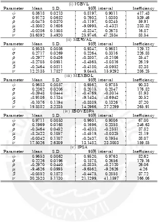
Table 3. MCMC Estimation Results of the SVSKt Model for Latin American Stock Return Data (i) IGBVL

Parameter Mean S.D. 95% interval Ine¢ciency

0.8618 0.0213 [ 0.8197, 0.9011 ] 417.43

0.9173 0.0682 [ 0.7602, 1.0380 ] 539.46

-0.0475 0.0370 [ -0.1197, 0.0245 ] 59.91

-8.8002 0.1686 [ -9.0995, -8.4321 ] 233.32

-0.0286 0.1508 [ -0.3247, 0.2678 ] 16.87

35.6892 5.4920 [ 25.9746, 47.2584 ] 88.54

(ii) MERVAL

Parameter Mean S.D. 95% interval Ine¢ciency

0.9535 0.0086 [ 0.9347, 0.9681 ] 129.12

0.2717 0.0269 [ 0.2264, 0.3316 ] 226.88

-0.2977 0.0436 [ -0.3807, -0.2106 ] 35.47

-8.2705 0.0951 [ -8.4565, -8.0816 ] 26.19

-0.2464 0.0811 [ -0.4180, -0.0952 ] 82.38

12.2135 1.7827 [ 9.0445, 15.9292 ] 286.25

(iii) MEXBOL

Parameter Mean S.D. 95% interval Ine¢ciency

0.9683 0.0057 [ 0.9562, 0.9785 ] 90.33

0.2362 0.0206 [ 0.2015, 0.2847 ] 176.82

-0.3948 0.0444 [ -0.4769, -0.3014 ] 81.93

-8.9186 0.1134 [ -9.1434, -8.6942 ] 30.52

-0.1076 0.1194 [ -0.3389, 0.1326 ] 37.20

19.8882 3.2235 [ 14.2966, 27.2299 ] 265.91

(iv) IBOVESPA

Parameter Mean S.D. 95% interval Ine¢ciency

0.9711 0.0053 [ 0.9601, 0.9806 ] 67.00

0.1969 0.0168 [ 0.1696, 0.2358 ] 246.63

-0.3464 0.0452 [ -0.4333, -0.2551 ] 37.82

-8.2422 0.1057 [ -8.4519, -8.0325 ] 21.19

-0.0342 0.1107 [ -0.2437, 0.1954 ] 38.07

17.5026 2.6309 [ 13.1482, 23.3003 ] 159.85

(v) IPSA

Parameter Mean S.D. 95% interval Ine¢ciency

0.9653 0.0062 [ 0.9520, 0.9763 ] 82.62

0.2226 0.0196 [ 0.1878, 0.2656 ] 179.16

-0.2970 0.0440 [ -0.3835, -0.2120 ] 26.06

-9.4626 0.0995 [ -9.6562, -9.2626 ] 4.26

-0.0852 0.1872 [ -0.4475, 0.2858 ] 37.72

The posterior means of , that measures the correlations between t and t, are estimated to be

negative for all indices considered. When values are negative, it implies that there exist leverage e¤ects. MEXBOL and IBOVESPA have in absolute value the highest posterior mean estimates of ( 0:3948and 0:3464, respectively), which imply that the leverage e¤ect is more notable for these indices. Also the 95% credible intervals are negative implying that the posterior probability that is negative is greater than 0:95, and the negativity of is credible. The same applies with MERVAL and IPSA (posterior mean estimates for are 0:2977and 0:2970;respectively) where the95% credible intervals are negative, but it is a minor leverage e¤ect than the previous indices. In the case of IGBVL, the posterior mean estimate of is also negative although very close to zero and the 95% credible intervals contain zero and positive values. This implies that the posterior distribution of ;although mainly located in the negative range, can take positive values or even zero, which would imply the non-existence of the leverage e¤ect in IGBVL returns. These results support the evidence of the leverage e¤ects in Latin American stock returns data.

Regarding the parameter , the posterior mean estimates of show that all indices have similar estimates in the range from0:1969to 0:2717 with the exception of the IGBVL returns, where the posterior mean estimate of takes a very high value (0:9173) compared to the other indices. This implies that the variance of the shock _tis large and the log-volatility has more variability than the other stock indices in Latin American. Regarding the posterior mean of , all indices show similar results in the range of 19:4626to 8:2422:

As mentioned previously, the skewness and the heavy tailedness of the GH Skew Student’s t-Distribution are determined jointly by the combination of the parameter values of and . With …xed, a lower value of implies a more negative skewness or left-skewness as well as heavier tails. On the other hand, with …xed, as becomes larger the density becomes less skewed and has lighter tails. The posterior means of are estimated to be negative for all indices returns data considered. MERVAL has the less value of posterior mean estimate of with 0:2464 and the 95% credible intervals are negative implying that the posterior probability that is negative is greater than 0:95, and the negativity of is credible. However, the posterior mean estimates of for IGBVL, MEXBOL, IBOVESPA and IPSA are also negative but the 95% credible intervals contain zero and positive values. We know that when = 0 in the SVSKt model correspond to symmetric student’s t-density. The estimates of are very close to zero for IGBVL, IBOVESPA and IPSA, it could imply the case of symmetric heavy tailed disturbances. Finally, the posterior means of are around 35:6892for IGBVL, 12:2135for MERVAL, 19:8882 for MEXBOL,17:5026 for IBOVESPA and 30:2523for IPSA returns.

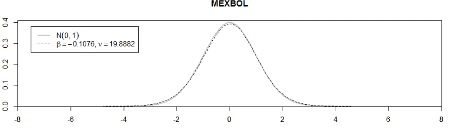
Figures 9-13 show the density of the GH Skew Student’s t-distribution with the estimates

Figure 9. Density of the GH Skew Student’st-distribution with estimates parameters = 0:0286and

= 35:6892for IGBVL data (Peru).

Figure 10. Density of the GH Skew Student’s t-distribution with estimates parameters = 0:2464and

= 12:2135for MERVAL data (Argentina).

Figure 11. Density of the GH Skew Student’st-distribution with estimates parameters = 0:1076and

Figure 12. Density of the GH Skew Student’st-distribution with estimates parameters = 0:0342and

= 17:5026for IBOVESPA data (Brazil).

Figure 13. Density of the GH Skew Student’st-distribution with estimates parameters = 0:0853and

= 30:2523for IPSA data (Chile).

Table 4. Estimation Results of the SVSKt Model for US S&P500 Stock Return Data

S&P500

Parameter Mean S.D. 95% interval Ine¢ciency

0.9703 0.0040 [ 0.9622, 0.9778 ] 40.86

0.2382 0.0135 [ 0.2125, 0.2652 ] 89.75

-0.6864 0.0323 [ -0.7449, -0.6199 ] 76.70

-9.4186 0.1001 [ -9.6135, -9.2207 ] 7.79

-0.7842 0.1899 [ -1.1837, -0.4380 ] 116.81

24.8685 3.8282 [ 18.2556, 33.5375 ] 189.21

Figure 14. Density of the GH Skew Student’st-distribution with estimates parameters = 0:7842and

= 24:8685for S&P500 data (US).

The indicator of how well MCMC chain mixes is measured by the ine¢ciency factor of the MCMC algorithm de…ned by 1 + 2 1_{s=1 s} as mentioned before. The ine¢ciency factor shows high values for parameters ; and for IGBVL. These results are supporting by the initial

MCMCFigure 3 that shows high autocorrelation through iterations of parameters ; and for

IGBVL that decay slowly. MERVAL, MEXBOL, IBOVESPA and IPSA returns show low values of ine¢ciency factor in all parameters estimates but parameter and v have higher values of ine¢ciency factor compared with the other parameters. In general, the ine¢ciency factor for the parameters of the S&P500 returns have low values.

Figure 15shows the log-volatility estimates for the Latin American stock indices returns

Figure 15. Log-volatility for IGBVL (2001/01/02 - 2013/12/30) and MERVAL, MEXBOL, IPSA, IBOVESPA and S&P500 (1996/01/02 - 2013/12/30) daily returns.

3.3 Model Comparison

In this subsection, model comparison between competing models for the daily stock returns are provided. We make a comparison between the SVSKt model with the SVt model (with symmetric Student’st-disturbances, or equivalently the SVSKt model with = 0). All models compared are allowed to include leverage e¤ects. Model comparison in a Bayesian framework can be performed using posterior odds. Ify=_fy_tgn_t=1 denote the returns observation vector; then, the posterior odds in favor of modelA,MA, to modelB,MB, is given by:

f(M_Ajy) f(M_Bjy) =

f(y_jMA)

f(y_jMB)

f(MA)

f(MB)

; (18)

wheref(M_ijy) is the posterior probability of the modeliwithi=A; B,f(Mi) is the prior

proba-bility of the model, f(y_jMi) is the marginal likelihood. _f(yf(y_jj_MM_BA₎) and _ff(M_(MA_B)₎ are called Bayes factor

and prior odds, respectively. As is the usual practice, the prior odds is assumed to be 1, that is the prior probabilities are assumed to be equal between competing models, so that the posterior odds ratio is equal to the Bayes factor (Asai, 2009). The idea is compare the competing models using their posterior probabilities to select the one that is the best supported by the data. We choose the model that yields the largest posterior probability, or equivalently the largest marginal likelihood. Thus, we choose the modelA if the posterior odds or Bayes factor is greater than 1, and we choose the model B if it is less than 1.

The marginal likelihood is de…ned by:

f(y_jMi) = Z

this is, the integral of the likelihood with respect to the prior density of the parameter. To compute the logarithm of the marginal likelihood, we follow the log marginal likelihood identity of model Mi which is developed in Chib(1995), and that can be written as:

logf(y_jMi) = logf(yjMi; i) + logf( ijMi) logf( ijMi; y); i=A; B; (20)

where i is the set of unknown parameters for modelMi,f(yjMi; i) is the likelihood of the model,

f( ijMi) is the prior probability density, andf( ijMi; y) is the posterior probability density. The

identity (20) holds for any value of i, but following Chib (1995), Kim et al. (1998), Asai (2009), Nakajima(2012) andNakajima and Omori(2012), we set i at its posterior mean calculated using

the MCMC samples to obtain a stable estimate of f(y_jMi). The prior probability density can

be easily calculated, although the likelihood and posterior part must be evaluated by simulation (Nakajima and Omori,2012). The likelihood f(y_jMi; i) can be estimated using the particle …lter

(see, for example, Pitt and Shephard (1999), Chib et al. (2002) and Omori et al. (2007)). For the posterior probability density f( _ijMi; y), it can be estimated using the method developed by Chib(1995) and Chib and Jeliazkov(2001) using samples obtained through additional but reduced iterations of the MCMC algorithm.

First, we estimate de SVt model. Figures16 20 show the MCMC estimation results of the SVt model for IGBVL, MERVAL, MEXBOL, IBOVESPA and IPSA stock returns data.

0 3 0 0 6 0 0 9 0 0 0

1 φ

0 3 0 0 6 0 0 9 0 0 0

1 σ

0 3 0 0 6 0 0 9 0 0 0

1 ρ

0 3 0 0 6 0 0 9 0 0 0

1 µ

0 3 0 0 6 0 0 9 0 0 0

1 ν

0 1 0 0 0 0 2 0 0 0 0 0 .8 0

0 .8 5 0 .9 0 0 .9 5 φ

0 1 0 0 0 0 2 0 0 0 0 0 .8

1 .0 1 .2

σ

0 1 0 0 0 0 2 0 0 0 0 -0 .1

0 .0 0 .1 ρ

0 1 0 0 0 0 2 0 0 0 0 -9 .0

-8 .5 -8 .0 µ

0 1 0 0 0 0 2 0 0 0 0 3 0

4 0 5 0 6 0 ν

0 .8 0 .8 5 0 .9 0 .9 5 1 0

2 0

φ

0 .7 5 1 1 .2 5 2

4

σ

-0 .2 -0 .1 0 0 .1 5

1 0

ρ

-9 -8 .5 -8 1

2

µ

2 0 4 0 6 0 0 .0 2 5

0 .0 5 0 0 .0 7 5 ν

0 3 0 0 6 0 0 9 0 0 0

1 φ

0 3 0 0 6 0 0 9 0 0 0

1 σ

0 3 0 0 6 0 0 9 0 0 0

1 ρ

0 3 0 0 6 0 0 9 0 0 0

1 µ

0 3 0 0 6 0 0 9 0 0 0

1 ν

0 1 0 0 0 0 2 0 0 0 0 0 .9 4

0 .9 6 0 .9 8 φ

0 1 0 0 0 0 2 0 0 0 0 0 .2 5

0 .3 0 0 .3 5

σ

0 1 0 0 0 0 2 0 0 0 0 -0 .4

-0 .3 -0 .2

ρ

0 1 0 0 0 0 2 0 0 0 0 -8 .5 0

-8 .2 5 -8 .0 0

µ

0 1 0 0 0 0 2 0 0 0 0 1 0

1 5 2 0 2 5 ν

0 .9 2 50 .9 50 .9 7 5 2 0

4 0

φ

0 .2 5 0 .3 5 5

1 0 1 5

σ

-0 .4 -0 .3 -0 .2 -0 .1 2 .5

5 .0 7 .5 1 0 .0 ρ

-8 .5-8 .2 5 -8 -7 .7 5 2

4

µ

1 0 2 0 0 .1

0 .2

ν

Figure 17. MCMC estimation results of the SVt model for MERVAL data (Argentina). Sample autocorrelations (top), sample paths (middle) and posterior densities (bottom).

0 3 0 0 6 0 0 9 0 0 0

1 φ

0 3 0 0 6 0 0 9 0 0 0

1 σ

0 3 0 0 6 0 0 9 0 0 0

1 ρ

0 3 0 0 6 0 0 9 0 0 0

1 µ

0 3 0 0 6 0 0 9 0 0 0

1 ν

0 1 0 0 0 0 2 0 0 0 0 0 .9 6

0 .9 8

φ

0 1 0 0 0 0 2 0 0 0 0 0 .2 0

0 .2 5 0 .3 0 0 .3 5 σ

0 1 0 0 0 0 2 0 0 0 0 -0 .5

-0 .4 -0 .3

ρ

0 1 0 0 0 0 2 0 0 0 0 -9 .2 5

-9 .0 0 -8 .7 5

µ

0 1 0 0 0 0 2 0 0 0 0 1 5

2 5

ν

0 .9 2 5 0 .9 5 0 .9 7 5 2 5

5 0 7 5

φ

0 .2 5 0 .3 5 1 0

2 0

σ

-0 .6-0 .5-0 .4-0 .3-0 .2 2 .5

5 .0 7 .5

ρ

-9 .5 -9 -8 .5 1

2 3 4 µ

1 0 2 0 3 0 0 .0 5

0 .1 0

ν

0 3 0 0 6 0 0 9 0 0 0

1 φ

0 3 0 0 6 0 0 9 0 0 0

1 σ

0 3 0 0 6 0 0 9 0 0 0

1 ρ

0 3 0 0 6 0 0 9 0 0 0

1 µ

0 3 0 0 6 0 0 9 0 0 0

1 ν

0 1 0 0 0 0 2 0 0 0 0 0 .9 4

0 .9 6 0 .9 8 φ

0 1 0 0 0 0 2 0 0 0 0 0 .2 5

0 .3 0

σ

0 1 0 0 0 0 2 0 0 0 0 -0 .4

-0 .3 -0 .2

ρ

0 1 0 0 0 0 2 0 0 0 0 -8 .4

-8 .2 -8 .0

µ

0 1 0 0 0 0 2 0 0 0 0 2 0

3 0

ν

0 .9 2 5 0 .9 5 0 .9 7 5 2 5

5 0

φ

0 .2 0 .2 5 0 .3 0 .3 5 1 0

2 0

σ

-0 .5-0 .4-0 .3-0 .2-0 .1 2 .5

5 .0 7 .5 1 0 .0 ρ

-8 .5 -8 .2 5 -8 2

4

µ

1 0 2 0 3 0 0 .0 5

0 .1 0

ν

Figure 19. MCMC estimation results of the SVt model for IBOVESPA data (Brazil). Sample autocorrelations (top), sample paths (middle) and posterior densities (bottom).

0 3 0 0 6 0 0 9 0 0 0

1 φ

0 3 0 0 6 0 0 9 0 0 0

1 σ

0 3 0 0 6 0 0 9 0 0 0

1 ρ

0 3 0 0 6 0 0 9 0 0 0

1 µ

0 3 0 0 6 0 0 9 0 0 0

1 ν

0 1 0 0 0 0 2 0 0 0 0 0 .9 6

0 .9 8 φ

0 1 0 0 0 0 2 0 0 0 0 0 .2 0

0 .2 5 0 .3 0

σ

0 1 0 0 0 0 2 0 0 0 0 -0 .3

-0 .2

ρ

0 1 0 0 0 0 2 0 0 0 0 -9 .5 0

-9 .2 5 -9 .0 0 µ

0 1 0 0 0 0 2 0 0 0 0 2 0

3 0 4 0 5 0 ν

0 .9 4 0 .9 6 0 .9 8 2 5

5 0 7 5 φ

0 .1 5 0 .2 0 .2 5 0 .3 1 0

2 0

σ

-0 .4 -0 .3 -0 .2 -0 .1 2 .5

5 .0 7 .5 1 0 .0 ρ

-9 .5 -9 2

4

µ

3 0 5 0 0 .0 2 5

0 .0 5 0 0 .0 7 5

ν

Table 5 shows the MCMC estimation results of the posterior estimates of the SVt model: the posterior means, the standard deviation, the 95% credible intervals and the ine¢ciency factors for the IGBVL, MERVAL, MEXBOL, IPSA and IBOVESPA stock return data. The posterior means of estimates parameter are very similar to the SVSKt model.

In order to compare the competing models, we estimate the log marginal likelihoods,logf(y_jMi),

as follows: (i) the likelihood is estimated using the auxiliary particle …lter with 10 000 particles. It is replicated 10 times to obtain the standard error of the likelihood estimate as in Nakajima and Omori(2012), and (ii) the posterior probability density ( _ijMi; y) is evaluated through5 000

additional MCMC runs. Table 6 shows the estimates of the log marginal likelihoods and their standard errors. We choose the model that yields the largest log marginal likelihood. The SVSKt model outperforms the SVt model for IGBVL, MERVAL and IBOVESPA stock returns data and the SVt model outperforms the SVSKt model for MEXBOL and IPSA stock returns data. We can see that the GH Skew Student’s t-disturbance distribution in the SV model (SVSKt model) is successful in describing the distribution of the daily stock return data for Peru, Argentina and Brazil and the symmetric Student’st-disturbance distribution in describing the distribution of the daily stock return data for MEXBOL and IPSA.

3.4 Prior Sensitivity Analysis

In spite of the computational expense of implementing, prior sensitivity analysis is an important tool in Bayesian inference because is important to assess the in‡uence of the prior distribution on the …nal inference. In order to check prior sensitivity, the posterior distribution of parameters must be studied using a variety of prior distributions. As in Nakajima and Omori (2012), we are focusing on the skewness and heavy-taildness parameters, and , to check the robustness of the model. We focus only on these parameters because we have assumed the values commonly used in the previous literature for the prior distributions of ; ; and :

The prior sensitivity analysis take into account the following priors: Prior #1: N(0;1); Gamma(16;0:8)1( >4);

Prior #2: N(0;4); Gamma(16;0:8)1( >4); Prior #3: N(0;1); Gamma(24;0:6)1( >4); Prior #4: N(0;4); Gamma(24;0:6)1( >4); Prior #5: N(0;1); Gamma(1:2;0:03)1( >4);

the prior for from prior #1 or prior #2 to prior #5. The estimates of get larger (from 36 to 161) implying lighter tails but similar skewness. The estimates of standard deviations for and using the prior #5 are larger than the estimates using the prior #1 and #2.

Table 5. MCMC Estimation Results of the SVt Model for Latin American Stock Return Data (i) IGBVL

Parameter Mean S.D. 95% interval Ine¢ciency

0.8613 0.0209 [ 0.8183, 0.9024 ] 407.89

0.9823 0.0964 [ 0.7655, 1.1565 ] 634.21

-0.0382 0.0386 [ -0.1122, 0.0401 ] 104.68

-8.7154 0.1639 [ -9.0253, -8.3828 ] 156.46

36.1646 5.7485 [ 26.2375, 48.8401 ] 105.50

(ii) MERVAL

Parameter Mean S.D. 95% interval Ine¢ciency

0.9533 0.0081 [ 0.9358, 0.9674 ] 103.72

0.2707 0.0244 [ 0.2279, 0.3256 ] 197.98

-0.2810 0.0434 [ -0.3652, -0.1945 ] 52.60

-8.2351 0.0948 [ -8.4186, -8.0462 ] 20.95

12.3573 1.9107 [ 9.2705, 16.8398 ] 253.81

(iii) MEXBOL

Parameter Mean S.D. 95% interval Ine¢ciency

0.9694 0.0054 [ 0.9584, 0.9788 ] 74.32

0.2282 0.0178 [ 0.1973, 0.2661 ] 160.80

-0.4037 0.0471 [ -0.4951, -0.3126 ] 94.09

-8.9333 0.1122 [ -9.1537, -8.7119 ] 17.26

17.2837 3.2351 [ 12.0182, 24.5254 ] 280.95

(iv) IBOVESPA

Parameter Mean S.D. 95% interval Ine¢ciency

0.9564 0.0067 [ 0.9423, 0.9687 ] 59.67

0.2528 0.0176 [ 0.2219, 0.2912 ] 169.99

-0.3244 0.0447 [ -0.4091, -0.2330 ] 46.67

-8.2198 0.0907 [ -8.3970, -8.0400 ] 11.09

20.1754 3.1531 [ 14.8120, 26.9762 ] 245.94

(v) IPSA

Parameter Mean S.D. 95% interval Ine¢ciency

0.9649 0.0061 [ 0.9521, 0.9759 ] 85.17

0.2253 0.0205 [ 0.1899, 0.2718 ] 283.75

-0.2928 0.0438 [ -0.3754, -0.2059 ] 43.86

-9.4536 0.1004 [ -9.6466, -9.2478 ] 23.10

Table 6. Estimated Log Marginal Likelihoods (Log-ML)

(i) IGBVL

SVSKt 9812.000 (1.582)

SVt 9781.776 (1.557)

(ii) MERVAL

SVSKt 11469.963 (0.806)

SVt 11464.903 (0.684)

(iii) MEXBOL

SVSKt 13377.385 (0.580)

SVt 13380.232 (0.704)

(iv) IBOVESPA

SVSKt 11624.206 (0.996)

SVt 11614.349 (0.627)

(v) IPSA

SVSKt 14583.355 (0.557)

SVt 14586.065 (0.653)

*Standard errors of the log-ML in parentheses.

MERVAL estimates for( ; )are not a¤ected by changing the prior for from prior #1 to prior #2, neither from prior #3 to prior #4. However, the estimates of ( ; ) are a¤ected by altering the prior for from prior #1 to prior #3 (or from prior #2 to prior #4). The estimates of get smaller (from 0:25 to 0:42) and the posterior means of get larger (from 12 to 20), implying greater skewness and lighter tails. The posterior standard deviations become larger re‡ecting the increase in the dispersion of the prior distribution for :Given less information on given by prior #5, the estimates of ( ; ) are similar to the estimates obtained by using priors #1 and #2.

MEXBOL estimates for are not a¤ected by changing the priors considered. The estimates of are similar using the priors #1 - #5 (in the range from 0:1076 to 0:0753). However, the estimates of (estimates are similar using prior #1, #2 and #5) are a¤ected by altering the prior for from prior #1 to prior #3 (or prior #2 to prior #4). The estimates of get larger (from19:5 to27) from prior #1, #2 and #5 to prior #3 and #4, implying lighter tails but similar skewness using the priors #3 to #4. The posterior standard deviations become larger from priors #1 and #2 to priors #3 and #4 and the estimates of standard deviations using prior #5 is the same for comparing to priors #1 and #2 but larger for :

Regarding the IBOVESPA, the estimates for ( ; )are not a¤ected by changing the prior from prior #1 to prior #2 or to prior #5, however from prior #1, #2 or #5 to prior #3 (or from prior #1, #2 or #5 to prior #4) the estimates for( ; ) are largely a¤ected. The estimates of and get larger from 0:03 to0:07 and from 17:5 to 29 (average), respectively, implying a disturbance density that becomes less skewed and has lighter tails. The posterior standard deviations of ( ; ) become larger from prior #1, #2 or #5 to prior #3 (or from prior #1, #2 or #5 to prior #4).

Table 7. Prior sensitivity analysis for the SVSKt model

Prior #1 Prior #2 Prior #3 Prior #4 Prior #5

(i) IGBVL

-0.0286 (0.1508) -0.0287 (0.1489) -0.0274 0.3105

[-0.3247, 0.2678] [-0.3203, 0.2675] [-0.6400, 0.5881]

16.87 15.71 9.72

35.6892 (5.4920) 36.7286 (5.5969) 161.0542 56.3557

[25.9746, 47.2584] [26.5760, 48.3670] [76.0663, 297.5268]

88.54 114.07 291.47

(ii) MERVAL

-0.2464 (0.0811) -0.2588 (0.0847) -0.4123 (0.1556) -0.4222 (0.1507) -0.2522 (0.0826)

[-0.4180, -0.0952] [-0.4372, -0.1019] [-0.7668, -0.1460] [-0.7691, -0.1748] [-0.4309, -0.1076]

82.38 73.46 106.15 146.31 91.94

12.2135 (1.7827) 12.4566 (1.8322) 20.1648 (4.5284) 19.0319 (4.2291) 11.1433 (1.8805)

[9.0445, 15.9292] [9.4167, 16.4069] [12.9397, 30.7610] [12.7557, 28.7367] [8.0934, 15.0799]

286.25 320.19 379.97 410.92 309.20

(iii) MEXBOL

-0.1076 (0.1194) -0.1008 (0.1110) -0.0818 (0.1559) -0.0753 (0.1574) -0.0855 (0.1194)

[-0.3389, 0.1326] [-0.3168, 0.1224] [-0.3795, 0.2325] [-0.3754, 0.2402] [-0.3099, 0.1692]

37.20 36.08 40.87 50.87 59.73

19.8882 (3.2235) 18.1714 (3.0561) 27.6532 (5.1416) 26.5082 (5.0933) 19.5090 (5.3784)

[14.2966, 27.2299] [13.4678, 25.6527] [19.1554, 39.1847] [17.7599, 38.1351] [12.7685, 34.4924]

265.91 260.93 287.83 270.82 469.37

(iv) IBOVESPA

-0.0342 (0.1107) -0.0374 (0.1137) 0.0774 (0.2088) 0.0649 (0.1915) -0.0366 (0.1273)

[-0.2437, 0.1954] [-0.2449, 0.2044] [-0.3077, 0.5243] [-0.2755, 0.4832] [-0.2672, 0.2518]

38.07 44.98 50.19 63.74 94.28

17.5026 (2.6309) 17.6462 (3.0990) 31.4925 (6.4575) 28.3000 (5.6489) 18.6492 (4.5117)

[13.1482, 23.3003] [12.7563, 24.9240] [19.5521, 46.0880] [19.3273, 40.6572] [13.0256, 30.7739]

159.85 276.67 309.95 252.38 396.59

(v) IPSA

-0.0852 (0.1872) -0.0891 (0.1957) -0.0808 (0.2880) -0.1129 (0.2703) -0.1381 (0.4383)

[-0.4475, 0.2858] [-0.4835, 0.2834] [-0.6762, 0.4567] [-0.6307, 0.4476] [-1.0289, 0.7027]

37.72 56.60 56.82 25.53 36.74

30.2523 (5.1130) 30.2391 (4.7554) 49.2582 (8.4254) 50.6228 (9.0323) 106.4110 (36.9622)

[21.1299, 41.1597] [22.2936, 40.9700] [34.8189, 67.3309] [35.1501, 70.4570] [48.2143, 189.1728]

166.06 187.32 115.43 194.78 327.33

As inNakajima and Omori(2012), we also observed that the posterior estimate of is sensitive to the choice of the prior distribution for and the posterior estimate of is also sensitive to the choice of the prior distribution for because the skewness and heavy-tailedness of the GH skew Student’st-distribution are determined by and simultaneously and not individually.

4 Conclusions

In this paper, we estimate a SV model incorporating both leverage e¤ects and skewed heavy-tailed disturbances taking into account theGH Skew Student’s t-distribution for a set of Latin American stock market indices using the Bayesian estimation method proposed by Nakajima and Omori

(2012). We apply the SVSKt model to daily returns of …ve Latin American stock market indices: IGBVL, MERVAL, MEXBOL, IPSA and IBOVESPA and we also analyze the U.S. S&P500 returns to compare the results. The SVSKt model can be considered a ‡exible model to …t the returns and volatility characteristics because the SVSKt model is able to model substantially skewed and heavy tailed data and includes the SV model with Normal disturbances (SV-Normal) and the SV model with symmetric Student’s t-disturbances (SVt).

The MCMC estimation results of the SVSKt model show that the sample paths of the iterations of parameters are stable, and the proposed estimation scheme works well for all indices except for the IGBVL (the Markov chains do not converge and there is high autocorrelation between iterations). The posterior mean parameter estimates are consistent with literature that indicate the high persistence of the volatility in stock returns. However, the results show that the IGBVL returns have low persistence in comparison to the volatility of the others stock indices of Latin American considered.

The results support the evidence that there are leverage e¤ects in all indices considered but there is not enough evidence for the IGBVL. The estimates show that the leverage e¤ect is more notable in MEXBOL and IBOVESPA, followed by MERVAL and IPSA. In the case of the IGBVL, the posterior mean estimate of is also negative but very close to zero, which would imply the non-existence of the leverage e¤ect in IGBVL returns. Another important result is that the log-volatility of IGBVL returns have more variability than the other stock returns in Latin American. Also, the results support the evidence of skewed heavy-tailed disturbances only for the MERVAL, symmetric heavy-tailed disturbances for the MEXBOL, IBOVESPA and IPSA, and symmetric Normal disturbances for the IGBVL.

Appendix

A. The GH _{Skew Student t-Distribution}

This appendix includes some important properties of the GH skew Student-t distribution. For a more complete treatment, seePrause(1999), Eberlein and Hammerstein (2004) and Aas and Ha¤

(2006). The GH Skew Studentt-Distribution is a limiting case of the GH distribution, which was introduced in Barndor¤-Nielsen (1977). The univariateGH distribution can be parameterized in several ways. Following,Prause(1999),Eberlein and Hammerstein(2004) andAas and Ha¤(2006), the probability density function of a GH random variablex is given by:

fGH(x; ; ; ; x; ) =

( 2 2) =2K 1 2

q

2_{+ (x}

x)2 exp ( (x x))

p

2 12 K

p

2 2 q 2_{+ (x}

x)2 1 2

(A.1)

whereKj is the modi…ed Bessel function7 of the third kind of orderjand x2R: >0determines

the shape, 0 _{j j}< determines the skewness, _{x 2}R is a location parameter and >0 serves for the scaling. ₂Rcharacterizes certain subclasses and considerably in‡uences the size of mass contained in the tails . The parameters must satisfy the conditions:

7_{The modi…ed Bessel function of the third kind with orderj, which we denote as}

Kj( ), has the integral represen-tation:

Kj(x) =

1 2

Z 1

0

w 1exp 1

2x(w+w 1

)dw ; x >0:

Some properties ofKj( ), taken fromAbramowitz and Stegun(1972), are:

Kj(x) =K j(x),

An asymptotic relations for small argumentsxis given by :

Kj(x) (j)2j 1x j asx!0andj >0;

Kj(x) ( j)2 j 1xjasx!0andj <0;

K0(x) ln(x):

An asymptotic relation for large argumentsxis given by:

Kj(x)

r

2xexp( x)asx! 1:

Ifj=n+1

2; n2Z;Kj can be calculated as follows:

Kn+1 2(x) =

r

2xexp( x) "

1 +

n

X

i=1

(n+i)! (n i)!i!(2x)

i

#

; n2N_;

0;_{j j}< if >0; (A.2) > 0;_{j j}< if = 0;

> 0;_{j j} if <0: The tails of theGH distribution behave as:

fGH(x) constjxj 1exp( jxj+ x) as x! 1; 8 ; (A.3)

hence, as long as _{j j 6}= ;theGH distribution has two semiheavy tails.

TheGH distribution may be represented as a Normal mean-variance mixture with Generalized Inverse Gaussian (GIG) distribution as a mixing distribution. This means that a GH variable X can be represented as:

X= _X + Z+pZ ; N(0;1); Z GIG( ; ; ); (A.4) with and Z independent and =p 2 2_{. It follows from (A.4) that X}

jZ = z N( _X + Z; Z). The density of theGIG distribution is given by:

fGH(z; ; ; ) =

z 1

2K ( )exp( 1 2(

2_z 1₊ 2_{z)): (A.5)}

Letting = =2( > 0) and _{! j j} in equation (A.1) (this is = 0), we obtain the GH

Skew Studentt-Distribution. Its probability density function is given by:

fGHskewt(x; ; ; x; ) =

212 j j +1

2 _{K +1}

2

r

2 2_{+ (x}

x)2 exp ( (x x))

(₂)p

q

2_{+ (x} x)2

+1 2

; ₆= 0;

(A.6) and

fGHskewt(x; ; ; !) =

( +1₂ )

p

(₂)

"

1 +(x x)

2

2

# ( +1)=2

; = 0: (A.7)

where (:) is the gamma function. The density fGHskewt(!; ; ; !) in (A.7) is known as the

The …rst four moments of a GH skew Studentt-distributed random variable X are:

E(X) = +

2

2; (A.8)

V ar(X) = 2

2 4

( 2)2_{( 4)}+ 2

2; (A.9)

Skewness(X) = 2( 4)

1=2

2 2 2+ ( 2)( 4) 3=2 3( 2) + 8 2 2

6 ; (A.10)

Kurtosis(X) = 6

2 2 2+ ( 2)( 4) 2 (A.11)

( 2)2( 4) + 16

4 2_{( 2)( 4)}

6 +

8 4 4(5 22) ( 6)( 8) :

We observe that for the mean and variance to exist, >2 and >4, respectively. The variance is only …nite when > 4, as opposed to the symmetric Student’s t-distribution. Skewness and (excess) kurtosis are de…ned only if >6and >8, respectively.

It follows from equation (A.3) that in the tails, the GH skewt-density is given by:

fGHskewt(x) constjxj =2 1exp( j xj+ x) asx! 1; (A.12)

Thus we have a heavy tail decaying as:

fGHskewt(x) constjxj =2 1 if

n _{<0and x}

! 1

>0and x_!+₁ ; (A.13) and a light tail decaying as

fGHskewt(x) constjxj =2 1exp( 2j xj)if

n _{<0and x}

!+₁

>0and x_{! 1} : (A.14) Thus the GH skewt-distribution has one heavy and one semiheavy tail. The heavy tail shows polynomial and the light tail exponential behavior. It is the only member ofGH family of distribu-tions having this property. Thus the GH skew studentt-distribution is able to model substantially skewed and heavy tailed data, as found for example in …nancial markets. The tails of theGH skew student t-distribution are characterized uniquely by parameters and , which determine jointly the degree of skewness and heavy tailedness. Finally, note that the heavy tail of the GH skew studentt-distribution is heavier than the tails of the symmetric Studentt-distribution, which have two tails decaying as polynomials and decay as:

B. MCMC Algorithm for the SVSKt Model

This appendix includes each sampling step in detail of the MCMC algorithm proposed byNakajima and Omori (2012) for the SVSKt model. For the prior distributions of and ; they assume

N( ₀; 2₀) and N( ₀; 2₀).

B.1 Generation of the parameters ( , , , ) (steps 2–4)

Step 2. The conditional posterior probability density ( _j ; ; ; ; ; h; z; y)( ( _j))is

( _j:) _/ ( )

q

1 2exp

(

(1 2)h2₁ 2 2

n 1 X

t=1

(ht+1 ht yt)2

2 2₍₁ 2₎ )

/ ( )

q

1 2exp

(

( )2

2 2

)

; (A.16)

where ht = ht , yt = (yte ht=2 zt)=pzt, zt = zt z, =

Xn 1

t=1

(ht+1 yt)ht

2_h2 1+

Xn 1

t=2 h2t

and

2 ₌ 2(1 2₎

2_h2 1+

Xn 1

t=2 h 2

t

.

In order to sample from this conditional posterior distribution,Nakajima and Omori(2012) im-plement the Metropolis–Hastings (MH) algorithm. They propose a candidate, T N_{( 1;1)}( ; 2_),

where T N(a;b)( ; 2) denotes the Normal distribution with mean and variance 2 truncated on

the interval(a; b). Then, they accept it with the probability given by min ( )

p 1 2 ( )p1 2 ;1 :

Step 3. Because the joint conditional posterior probability density (#_j ; ; ; h; z; y)( (#_j)) of # = ( ; )0 is given by (#_j) _/ (#) n(1 2)n21exp (1

2_)h2 1 2 2

Xn 1 t=1

(ht+1 ht yt)2

2 2₍₁ 2₎ ;

a probability density from which it is not easy to sample. Nakajima and Omori (2012) ap-ply the MH algorithm based on a Normal approximation of the density around the mode. Be-cause there is a constraint, R = _f# : > 0; _{j j} < 1_g, on the parameter space of the poste-rior distribution, they consider the transformation # to ! = (!1; !2)0, where !1 = log , and

!2= log(1 + ) log(1 ), to generate a candidate using a Normal distribution. They …rst search

for#b that approximately maximizes (#_j:), and obtain its transformed value !_b. They next gener-ate a candidgener-ate ! N(! ; ), where ! =!_b+ @log_@!e(!j)

!=e! and

1 ₌ @2_loge(! j) @!@!0

!=e!;

where _e(!_j) is a transformed conditional posterior density. Then, they accept the candidate ! with probabilityminn (# j)fN(!j! ; )jJ(#)j

(#j)fN(! j! ; )jJ(# )j;1

o

;wherefN(xj ; )denotes the probability density