Comprehensive evaluation of a New GPU based approach to the shortest path problem

(1)

(will be inserted by the editor)

Comprehensive Evaluation of a New GPU-based

Approach to the Shortest Path Problem

Hector Ortega-Arranz · Yuri Torres · Arturo Gonzalez-Escribano ·

Diego R. Llanos

Received: date / Accepted: date

Abstract The Single-Source Shortest Path (SSSP) problem arises in many different fields. In this paper, we present a GPU SSSP algorithm implementa-tion. Our work significantly speeds up the computation of the SSSP, not only with respect to a CPU-based version, but also to other state-of-the-art GPU implementations based on Dijkstra. Both GPU implementations have been evaluated using the latest NVIDIA architectures. The graphs chosen as input sets vary in nature, size, and fan-out degree, in order to evaluate the behavior of the algorithms for different data classes. Additionally, we have enhanced our GPU algorithm implementation using two optimization techniques: The use of a proper choice of threadblock size; and the modification of the GPU L1 cache memory state of NVIDIA devices. These optimizations lead to performance improvements of up to 23% with respect to the non-optimized versions. In addition, we have made a platform comparison of several NVIDIA boards in order to distinguish which one is better for each class of graphs, depending on their features. Finally, we compare our results with an optimized sequential implementation of Dijkstra’s algorithm included in the reference Boost library, obtaining an improvement ratio of up to 19× for some graph families, using less memory space.

Keywords Dijkstra·GPGPU· Kernel characterization· NVIDIA platform comparison·Optimization techniques·SSSP·Boost Library

1 Introduction

Many problems that arise in real-world networks imply the computation of the shortest paths, and their distances, from a source to any destination point. Some examples include navigation systems [1], spatial databases [2],

Hector Ortega-Arranz·Yuri Torres·Arturo Gonzalez-Escribano·Diego R. Llanos Departamento de Inform´atica, Universidad de Valladolid, Spain.

Tel.: (+34) 983.423.000 Ext. 5642

(2)

and web searching [3]. Algorithms to solve shortest-path problems are compu-tationally costly. Thus, in many cases, commercial products implement heuris-tic approaches to give approximate solutions instead. Although heurisheuris-tics are usually faster and do not need a great amount of data storage, they do not guarantee the optimal path.

The Single-Source Shortest Path (SSSP) problem is a classical problem of optimization. Given a graph G = (V, E), a function w(e) : e ∈ E that associates a weight to the edges of the graph, and a source nodes, the prob-lem consists of computing the paths (sequence of adjacent edges) with the smallest accumulated weight froms to every nodev∈V. The classical algo-rithm that solves the SSSP problem is Dijkstra’s algoalgo-rithm [4]. Wheren=|V| and m=|E|, the complexity time of this algorithm isO(n2_{). This}

complex-ity is reduced to O(m+nlogn) when special data structures are used, as with the implementation of Dijkstra’s algorithm included in the Boost Graph Library [5] which exploits the relaxed-heap structures. The efficiency of Di-jkstra’s algorithm is based on the ordering of previously computed results. This feature makes its parallelization a difficult task. However, under certain situations, this ordering can be permuted without leading to wrong results or performance losses.

An emerging method of parallel computation includes the use of hardware accelerators, such as graphic processing units (GPUs). Their powerful capabil-ities have triggered their massive use to speed up highly parallel computations. The application of GPGPU (General Purpose computing on GPUs) to accel-erate problems related with shortest-path problems has increased during the last few years. Some GPU solutions to the SSSP problem have been previously developed using different algorithms, such as Dijkstra’s algorithm in [6, 7].

GPGPU programming has been simplified by the introduction of high-level data parallel languages, such as CUDA [8]. A CUDA application has some configuration and execution parameters, such as the threadblock size, and the L1 cache state, whose combined use can lead to significant performance gains.

In this paper, we present an adapted version of Crauser’s algorithm [9] for the GPU architectures and an experimental comparison with both its se-quential version on CPU and the parallel GPU implementations of Mart´ınet al. [6]. Additionally, we have enhanced the performance of the fastest meth-ods by applying two CUDA optimization techniques: A proper selection of the threadblock size, and the configuration of the L1 cache memory. We have used the latest CUDA architectures (Fermi GF110, Kepler GK104, and Kepler GK110) and we have made a comparison of them in order to distinguish which one is better for each kind of graph. Finally, we have compared our results with the implementation of Dijkstra’s algorithm of the Boost library.

The rest of this paper is organized as follows. Section 2 briefly describes both the Dijkstra’s sequential algorithm and some proposed parallel implemen-tations. Section 3 explains in depth our GPU-implementation of the Crauser

et al. algorithm and the Mart´ınet al.CUDA solution for the SSSP problem.

(3)

✁ ✂

✄ ✄ ✂

☎

✆ ✝

✞

✁ ✂

✄ ✄ ✂

☎

✆ ✝

✞

✁ ✂

✄ ✄ ✂

☎

✆ ✝

✞

(a) (b) (c)

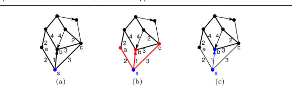
Fig. 1 Dijkstra’s algorithm steps: Initialization (a), edge relaxation (b), and settlement (c).

2 Dijkstra’s algorithm overview and related work

2.1 Dijkstra’s algorithm

Dijkstra’s algorithm constructs minimal paths from a source node s to the remaining nodes, exploring adjacent nodes following a proximity criterion. This exploring process is known as edge relaxation. When an edge (u, v) is relaxed from a node u, it is said that node v has been reached. Therefore, there is a path fromsthroughuto reachv with a tentative shortest distance. Nodev is considered settled when the algorithm finds the shortest path from source nodestov. The algorithm finishes when all nodes are settled.

The algorithm uses an array, D, that stores all tentative distances found from the source node, s, to the rest of the nodes. At the beginning of the algorithm, every node is unreached and no distances are known, soD[i] =∞ for all nodesi, except the current source nodeD[s] = 0. Note that the reached nodes that have not been settled yet and the unreached nodes are considered unsettled nodes. The algorithm proceeds as follows (see Fig. 1):

1. (Initialization) It starts on the source nodes, initializing the distance array D[i] =∞for all nodesiandD[s] = 0. Nodesis settled, and is considered as thefrontier node f (f ←s), the starting node for the edge relaxation. 2. (Edge relaxation) For every nodevadjacent tof that has not been settled

(nodes a,b, andc in Fig. 1), a new distance from source node s is found using the path through f, with value D[f] +w(f, v). If this distance is smaller than the previous value D[v], then D[v]←D[f] +w(f, v).

3. (Settlement) The non-settled nodebwith the minimal value inD is taken as the new frontier node (f ←b), and it is now considered as settled. 4. (Termination criterion) If all nodes have been settled, the algorithm

fin-ishes. Otherwise, the algorithm proceeds once more to step 2.

2.2 Dijkstra with priority queues

The most efficient implementations of Dijkstra’s algorithm, for sparse graphs (graphs withm << n2_{), have a priority queue to store the reached nodes [10].}

(4)

restrictions. This relaxed-heap structure is used in the optimized sequential implementation of Dijkstra’s algorithm of the Boost reference library.

2.3 Parallel versions of Dijkstra’s algorithm

We can distinguish two parallelization alternatives that can be applied to Dijkstra’s approach. The first one parallelizes the internal operations of the sequential Dijkstra algorithm, while the second one performs several Dijkstra algorithms through disjoint subgraphs in parallel [12]. This paper focuses on the first solution.

The key to the parallelization of a single sequential Dijkstra algorithm is the inherent parallelism of its loops. For each iteration of Dijkstra’s algorithm,

theouter loop selects a node to compute new distance labels. Inside this loop,

the algorithm relaxes its outgoing edges in order to update the old distance labels, that is, the inner loop. After these relaxing operations, the algorithm calculates the minimum tentative distance from the unsettled nodes set to extract the next frontier node.

Parallelizing theinner loop implies simultaneously traversing the outgoing edges of the frontier node. One of the algorithms presented in [13] is an example of this kind of parallelization. However, having only the outgoing edges of one frontier node, there is not enough parallelism to port this algorithm to the GPUs in order to properly exploit the huge number of cores.

Parallelizing theouter loopimplies computing in each iterationi, a frontier setFiof nodes that can be settled in parallel without affecting the algorithm’s correctness. The main problem here is to identify this set of nodes v whose tentative distances from sources,δ(v), are in reality the minimum shortest-distance,d(v). As the algorithm advances in the search, the number of reached nodes that can be computed in parallel increases considerably, fitting the GPU capabilities well. Some algorithms that are based on this idea are [9, 6]. ∆-Stepping is another algorithm [14] that also parallelizes the outer loop of the original Dijkstra’s algorithm, by exploring in parallel several nodes grouped together in a bucket. Several buckets are used to group nodes with different tentative distance ranges. On each iteration, the algorithm relaxes in parallel all the outgoing edges from all the nodes in the lowest range bucket. It first selects the edges that end on nodes inside the same bucket (light edges), and later the rest (heavy edges). Note that this algorithm can find that a processed node has to be recomputed if, at the same time, another node reduced the tentative distance of the first one, implying the bucket change of its reached nodes. The dynamic nature of the bucket structure and the fine-grain changes of node-bucket association do not fit well with the GPU features [15].

3 Parallel Dijkstra with CUDA

(5)

Algorithm 1GPU code of Crauser’s algorithm. 1: while(∆6=∞)do

2: gpu kernel relax(U, F, δ); //Edge relaxation 3: ∆=gpu kernel minimum(U, δ); //Settlement step 1 4: gpu kernel update(U, F, δ, ∆); //Settlement step 2 5: end while

3.1 Defining the frontier set

Dijkstra’s algorithm, in each iteration i, calculates the minimum tentative distance between all the nodes that belong to the unsettled set,Ui. After that, every unsettled node whose tentative distance is equal to this minimum value can be safely settled. These nodes that have been settled will be the frontier nodes of the following iteration, and their outgoing edges will be traversed to reduce the tentative distances of the adjacent nodes.

Parallelizing the Dijkstra algorithm requires the identification of which nodes can be settled and used as frontier nodes at the same time. Mart´ınet al.[6] insert into the following frontier set,Fi+1, all nodes with the minimum

ten-tative distance in order to process them simultaneously. Crauser et al. [9] introduce a more aggressive enhancement, augmenting the frontier set with nodes that have bigger tentative distances. The algorithm computes in each iterationi, for each node of the unsettled set,u∈Ui, the sum of: (1) its tenta-tive distance,δ(u), and (2) the minimum weight of its outgoing edges. Then, from among these computed values, it calculates the total minimum value, also called threshold. Finally, an unsettled node,u, can be safely settled, becoming part of the next frontier set, only if itsδ(u) is lower than or equal to the calcu-lated threshold. We name this threshold as∆i, that is the limit value computed in each iteration i, holding that any unsettled nodeuwithδ(u)≤∆i can be safely settled. The bigger the value of∆i, the more parallelism is exploited.

Our implementation follows the idea proposed by Crauseret al.[9] of incre-menting each∆i. For every node v∈V, the minimum weight of its outgoing edges, that is, ω(v) = min{w(v, z) : (v, z)∈E}, is calculated in a precompu-tation phase. For each iteration i, having all tentative distances of the nodes in the unsettled set, we compute∆i= min{(δ(u) +ω(u)) :u∈Ui}. Thus, it is possible to put into the frontier setFi+1 every nodev whoseδ(v)≤∆i.

3.2 Our GPU implementation: The successors variant

The four Dijkstra’s algorithm steps described in Sect. 2.1 can be easily trans-formed into a GPU general algorithm (see Alg. 1). It is composed of three kernels that execute the internal operations of the Dijkstra vertexouter loop. In therelax kernel (Alg. 2 (left)), a GPU thread is associated for each node in the graph. Those threads assigned to frontier nodes traverse their outgoing edges, reducing/relaxing the distances of their unsettled adjacent nodes.

The minimum kernel computes the minimum tentative distance of the

(6)

Algorithm 2Pseudo-code of therelax kernel(left) and theupdate kernel (right). gpu kernel relax(U, F,δ)

1: tid = thread.Id;

2: if (F[tid] == TRUE)then

3: for allj successor of tiddo

4: if(U[j] == TRUE)then

5: δ[j] =Atomicmin{δ[j], δ[tid] +w(tid, j)}; 6: end if

7: end for

8: end if

gpu kernel update(U, F,δ,∆) 1:tid = thread.Id;

2:F[tid]= FALSE;

3:if (U[tid]==TRUE)then

4: if (δ[tid]<=∆)then

5: U[tid]= FALSE; 6: F[tid]= TRUE; 7: end if

8:end if

code of this kernel is shown because, to accomplish this task, we have used

thereduce4 method included in the CUDA SDK [16], by simply inserting an

additional sum operation per thread before the reduction loop. The resulting value of this reduction is∆i.

The update kernel (Alg. 2 (right)) settles the nodes that belong to the

unsettled set,v∈Ui, whose tentative distance,δ(v), is lower than or equal to ∆i. This task extracts the settled nodes from Ui. The resulting set, Ui+1, is

the following-iteration unsettled set. The extracted nodes are added toFi+1,

the following-iteration frontier set. Each single GPU thread checks, for its corresponding node v, whether U(v)∧δ(v) ≤∆i. If so, it assigns v to Fi+1

and deletesv fromUi+1.

Besides the basic structures needed to hold nodes, edges, and their weights, three vectors are used to store node properties: (a)U[v], which stores whether a nodevis an unsettled node; (b)F[v], which stores whether a nodevis a frontier node; and (c)δ[v], which stores the tentative distance from source to nodev.

3.3 Mart´ın et al. successors and predecessors variants

In this subsection, we describe the GPU approach developed by Mart´ınet al.

[6]. In order to parallelize Dijkstra’s algorithm, they have introduced a conser-vative enhancement to increase the frontier set, inserting only the nodes with the same minimum tentative distance. According to our notation presented above, their frontier set of any iteration i, Fi+1, is composed of every node

x∈Ui with a tentative distanceδ(x) equal to∆i, in which∆i = min{δ(u) : u ∈Ui}. Their update kernel also differs from ours in the frontier-set check condition,U(v)∧δ(v) =∆i.

(7)

4 Experimental setup

In this section, we describe the methodology used to design and carry out experiments to validate our approach, the different scenarios we considered, and the platforms and input sets used.

4.1 Methodology

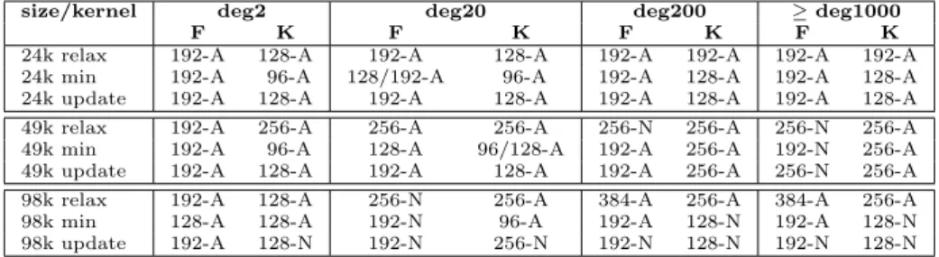
From the suite of different implementations described in [6], we used as refer-ences the sequential implementation (labeled here as CPU Mart´ın), and the fastest version fully implemented for GPUs (GPU Mart´ın). This means that we have left out the hybrid approaches that execute some phases on the CPU and others on the GPU. To fairly compare the performance gain of our algorithms, we used the same input set of synthetic graphs of Mart´ınet al.’s study (Mart´ın graphs), and the same CUDA configuration values they used: (1) 256 threads per block for all kernels; and (2) L1 cache normal state (16KB). We named this configuration thedefault configuration. On the other hand, the values used for our optimized implementation were taken from [17] (see Table 1).

As a second scenario, we have extended the experimentation for the result-ing best approach (the successors variant), testresult-ing it with synthetic random graphs generated using a technique described in [18], appropriate for generic random graph generation, and real-world graphs publicly available [19, 20].

For all studied scenarios, we have randomly selected 100 sources from the graph nodes, using uniform distribution, to solve 100 SSSP problems in order to obtain an average time. A description of each experiment is presented below:

1. Mart´ın graphs experimentation.

a. Sequential algorithmic comparison: CPU Mart´ın vs CPU Crauser

im-plementations for the successors and predecessors variants.

b. Parallel algorithmic comparison: GPU Mart´ın vs GPU Crauser

imple-mentations using both successors and predecessors variants.

c. Evaluation of the optimized version obtained by using the kernel

char-acterization values: CPU and GPU Crauser vs Optimized GPU.

d. Evaluation of the performance degradation due to the divergent branch

and dummy computations.

2. Synthetic and real-world graphs experimentation.

A. GPU parallel state-of-art improvement:GPU Mart´ın vs GPU Crauser,

and also the comparison vs its sequential version, CPU Crauser.

B. Evaluation of the optimized version obtained by using the kernel

char-acterization values: CPU and GPU Crauser vs Optimized GPU.

C. A GPU architectural comparison of the results obtained launching the

optimized GPU Crauser version on the different experimental boards (Fermi GF110, Kepler GK104, and Kepler GK110), and input sets.

D. Comparison of our GPU approach with a sequential state-of-art

ver-sion:Dijkstra’s algorithm of Boost library vs Optimized GPU Crauser,

(8)

Table 1 Values selected for threadblock-size and L1 cache state through kernel characteri-zation process for Fermi (F) and Kepler (K). L1 states are: (A) Augmented or (N) Normal.

size/kernel deg2 deg20 deg200 ≥deg1000

F K F K F K F K

24k relax 192-A 128-A 192-A 128-A 192-A 192-A 192-A 192-A 24k min 192-A 96-A 128/192-A 96-A 192-A 128-A 192-A 128-A 24k update 192-A 128-A 192-A 128-A 192-A 128-A 192-A 128-A 49k relax 192-A 256-A 256-A 256-A 256-N 256-A 256-N 256-A 49k min 192-A 96-A 128-A 96/128-A 192-A 256-A 192-N 256-A 49k update 192-A 128-A 192-A 128-A 192-A 256-A 256-N 256-A 98k relax 192-A 128-A 256-N 256-A 384-A 256-A 384-A 256-A 98k min 128-A 128-A 192-N 96-A 192-A 128-N 192-A 128-N 98k update 192-A 128-N 192-N 256-N 192-N 128-N 192-N 128-N

4.2 Target architectures

The performance results of the work of Mart´ınet al.were obtained using a pre-Fermi architecture. We replicated the experiments using three NVIDIA GPU devices, a GeForce GTX 480 (Fermi GF110), a GeForce GTX 680 (Kepler GK104), and a GeForce GTX Titan Black (Kepler GK110). For our experi-ments we named these devices Fermi, Kepler, and Titan boards, respectively. The host machine for the first two boards is an Intel(R) Core i7 CPU 960 3.20GHz, with a global memory of 6 GB DDR3. It runs an Ubuntu Desk-top 10.04 (64 bits) OS. The experiments were launched using the CUDA 4.2 toolkit. The host machine for the Titan board is an Intel(R) Xeon E5 2620 2.1GHz, with a global memory of 32GB DDR3 running an Ubuntu Server 14.04 (64 bits) operating system. The experiments have been launched using the CUDA 6.0 toolkit. The latter machine described is where the sequential CPU implementations have been carried out, because the Boost library imple-mentation needs big amounts of global memory to allocate the relaxed heap structure. All programs have been compiled with gcc using the -O3 flag, which includes the automatic vectorization of the code in the Xeon machine.

4.3 Input set characteristics

In this section, we describe the different input sets used for our experiments. The first one is from Mart´ınet al.. We used their graph creation tool with the aim of comparing our implementation with their solution. The second input set is composed by a collection of random graphs generated with a specific technique designed to produce random structures. The third input set contains real-world and benchmarking graphs provided by some research institutions. All the graphs of every input set used are stored using adjacency list structures.

Mart´ın’s graphs: These graphs have sizes that range from 220 _{to 11}_·

220 _{vertices. We kept the degree they chose (degree seven), so the generator}

tool creates seven adjacent predecessors for each vertex. They inverted the generated graphs in order to study approaches based on the successors version. The edge weights are integers that randomly range from 1 to 10.

(9)

in order to: (1) avoid dependences between a particular graph structure of the input sets and performance effects related to the exploitation of the GPU hardware resources; and (2) avoid focusing on specific domains, such as road maps, physical networks, or sensor networks among others, that would lead to loss of generality. In order to evaluate the algorithmic behavior for some graph features, we have generated a collection of graphs using three sizes (24 576, 49 152, and 98 304) and five fan-out degrees (2, 20, 200, 1 000, and 2 000). These sizes, smaller than Mart´ın’s graphs, were chosen with the aim of discovering the threshold where the sequential CPU version executes faster than the GPU. Weights are integers randomly chosen, and uniformly dis-tributed in the range [1. . .100].

Dimacs and social-network graphs: We used some of the real-world and benchmarking graphs facilitated by DIMACS [19], such as the walshaw graphs (low degree), clustering graphs (low degree), rmat-kronecker graphs (medium-high degree), and the social-networks graphs (medium degree), in-cluding also a graph based on the flickr structure provided by [20]. The purpose of experimenting with these graphs is to observe if the evaluated approaches not only performs well in synthetic laboratory graphs but also in real contexts.

4.4 Divergent Branch and dummy computation

CUDA Branch divergence, known asdivergent branch effect [8], has a signifi-cant impact on the performance of GPU programs. In the presence of a data dependent branch that causes different threads in the same warp to follow different execution paths, the warp serially executes each branch path taken.

The threads of the relax kernel, for bothpredecessors andsuccessors vari-ants, have a divergent branch. Two different kinds of threads are identified due to this divergent branch: (1)dummy threads, that do not make any com-putation for the assigned node, and (2) working threads, that carry out the relax operation from the assigned node. In order to discuss if the presence of such divergent branches causes a significant performance degradation, we have carried out an experiment to measure the efficiency ratio of the diver-gent branch, by means of the CUDA VisualProfiler. The presence of so many dummy threads in therelax kernelimplies too much futile computation. With the aim of knowing if it is possible to compute this kernel more efficiently, we have measured both the total number of executed threads and the number of

working threads.

5 Experimental results

(10)

0 5000 10000 15000 20000 25000

0 1 2 3 4 5 6 7 8 9 10 11 12

Time (ms)

Number of nodes (multiples of 220₎ CPU Martin vs. CPU Crauser

CPU Martin Pred CPU Crauser Pred CPU Martin Succ CPU Crauser Succ

0 500 1000 1500 2000

0 1 2 3 4 5 6 7 8 9 10 11 12

Time (ms)

Number of nodes (multiples of 220₎ GPU Martin vs. GPU Crauser

Fermi Martin Pred Kepler Martin Pred Kepler Crauser Pred Fermi Crauser Pred Fermi Martin Succ Kepler Martin Succ Kepler Crauser Succ Fermi Crauser Succ

(a) (b)

0 50 100 150 200 250 300

0 1 2 3 4 5 6 7 8 9 10 11 12

Time (ms)

Number of nodes (multiples of 220₎ Default GPU Crauser vs. Optimized GPU Crauser (Succ)

Kepler GPU Crauser Opt. Kepler GPU Crauser Fermi GPU Crauser Opt. Fermi GPU Crauser

1e+06 1e+07 1e+08 1e+09

0 1 2 3 4 5 6 7 8 9 10 11 12

#Threads (logscale)

Number of nodes (multiples of 220₎ Adjacency lists dummy computations

Total threads Working threads, Pred Working threads, Succ

(c) (d)

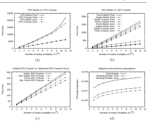
Fig. 2 Experimental results of Mart´ın’s graphs: Execution times of CPU-Mart´ın vs. our

CPU-Crauser (a), GPU-Mart´ın vs. our GPU-Crauser (b), and GPU-Crauser Successors vs its optimized version (c); and number of total threads vs. number of working threads in the

relax kernel(d).

5.1 Mart´ın’s graphs

a. CPU algorithmic comparison

Figure 2 (a) shows the execution times for both sequential algorithms: Mart´ın’s, and our approach. For each one, we present results for the two variants: Succes-sors and PredecesSucces-sors. Although all versions are sequential and no parallelism can be exploited, the fact of having more nodes in the frontier set per iteration for the Crauser algorithm means that fewer iterations are needed to complete the computation of the whole SSSP. This means that the minimum calculation and the updating operation are computed fewer times. The gain ranges from 4.44% to 18.34%, for Successors and Predecessors variants respectively.

b. GPU algorithmic comparison

(11)

one. The Fermi performance improvement, over Mart´ın’s algorithm, goes from 20.29%, for the Predecessors variant, up to 45.80%, for the Successors variant. On the other hand, these improvements are not so significant in the Kepler architecture, involving just 1.07% and 8.14% for Successors and Predecessors variants respectively.

c. GPU vs Optimized comparison

Figure 2 (c) shows the execution times for the fastest variant, the GPU Crauser Successors variant, using the default and the optimized configurations; both carried out in the Fermi and Kepler CUDA architectures. The use of optimiza-tion techniques, which take better advantage of the GPU hardware resources, leads to faster execution times of up to 9.75% for Fermi, and up to 5.11% for Kepler architectures. Comparing the execution times of this optimized GPU Crauser Successors with its analogous sequential version, the CPU Crauser Successors, we observe that the use of the GPU offers a speed-up of up to 26.68×, for Fermi’s architecture, and up to 21.4×, for Kepler’s architecture.

d. Divergent Branch and dummy computations

Figure 2 (d) shows the total number of executed threads and the number

of working threads in the relax kernel. In both cases, the number of working

threads is significantly lower than the total number of launched threads. The

percentage ofdummy threads vs. total threads varies from 90% for the prede-cessors variant, to 96% for the sucprede-cessors variant. The CUDA VisualProfiler results have shown that the efficiency ratio of the divergent branch in therelax

kernel is good, from 94.3% to 99.5%. Thus, the serialized work-flows in a warp,

due to the divergent branch, hardly affects the performance of this kernel. The execution ofdummy warps, that are warps of 32dummy threads, do not lead to the serializing of different work-flows, because all threads of these warps process the same dummy instruction. Therefore, having many more dummy

warps thanmixed warps, warps filled with bothdummy andworking threads,

implies that the performance is hardly affected by the divergent branch.

5.2 Synthetic random and real-world graphs

A. CPU and GPU algorithmic comparison

(12)

0 200 400 600 800 1000 1200 1400 1600

2 20 200 1000 2000

Time (ms)

Degree (logscale) random24k - SYNTH - CPU vs GPU

Martin Titan CPU Crauser Xeon Crauser Titan 0 500 1000 1500 2000 2500

2 20 200 1000 2000

Time (ms)

Martin Titan CPU Crauser Xeon Crauser Titan 0 500 1000 1500 2000 2500 3000 3500

2 5 10 20 50 100 200 500 1000 2000

Time (ms)

Martin Titan CPU Crauser Xeon Crauser Titan

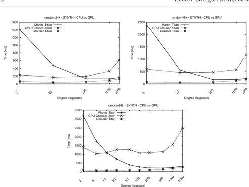
Fig. 3 Scenario A: Execution times of successors algorithmic variants (GPU Mart´ın,

CPU Crauser, and GPU Crauser) for synthetic random graphs.

10 100 1000 10000 100000

1114316386 45087 78136 99617 143437

Time (ms - logscale)

Nodes Walshaw - DIMACS - CPU vs GPU

Martin Titan CPU Crauser Xeon Crauser Titan 10 100 1000 10000 100000

16726 22963 31163 40421 192244 325557 862664

Nodes (logscale) Clustering - DIMACS - CPU vs GPU

100 1000 10000 100000

434102 540486 820878

Nodes Social Networks- DIMACS - CPU vs GPU

100 1000 10000 100000

65536131072262144 524288 1048576 2097152

Nodes Kronecker - DIMACS - CPU vs GPU

Fig. 4 Scenario A: Execution times, in logarithmic scale, of successors algorithmic variants

(13)

Table 2 Speedups of GPU Crauser vs the sequential implementation (CPU C), and vs GPU Martin (GPU M) for the used GPU boards. Speedups above 10×are highlighted in grey.

Fermi Kepler Titan

CPU C GPU M CPU C GPU M CPU C GPU M

24k deg2 5.90_× 24.61_× 5.54_× 24.66_× 3.56_× 21.62_× 24k deg20 6.07_× 11.04_× 5.98_× 11.23_× 4.33_× 12.11_× 24k deg200 3.84× 2.50× 3.94× 2.39× 3.49× 2.40× 24k deg1000 3.00× 1.43× 3.08× 1.40× 3.76× 1.48× 24k deg2000 3.30× 1.22× 3.51× 1.21× 4.66× 1.25× 49k deg2 10.78× 29.97× 10.47× 29.20× 7.39× 29.62× 49k deg20 10.55× 9.66× 10.63× 9.62× 7.76× 9.40× 49k deg200 5.93× 2.18× 6.32× 2.10× 6.26× 2.30× 49k deg1000 3.62_× 1.35_× 3.80_× 1.32_× 4.55_× 1.40_× 49k deg2000 4.85_× 1.20_× 4.98_× 1.18_× 6.39_× 1.19_× 98k deg2 18.42× 31.85× 18.01× 31,70× 14.22× 32.20× 98k deg20 17.33× 7.75× 17.63× 7.73× 14.97× 8.55× 98k deg200 8.23× 1.87× 9.07× 1.86× 10.18× 2.07× 98k deg1000 5.91× 1.27× 6.13× 1.24× 8.16× 1.31× 98k deg2000 6.23× 1.13× 6.32× 1.13× 9.09× 1.16×

Table 3 Best speedups obtained for each Dimacs family graph of GPU Crauser vs the

sequential implementation (CPU C), and vs GPU Martin (GPU M).

Fermi Kepler Titan

CPU C GPU M CPU C GPU M CPU C GPU M

walshaw 19.23_× 27.99_× 19.22_× 28.00_× 16.57_× 29.20_× clustering 25.43_× 23.97_× 26.68_× 26.63_× 25.41_× 30.61_× kronecker 27.09_× 3.78_× 30.76_× 4.05_× 43.05_× 5.21_× social net. 33.30_× 129.71_× 37.09_× 130.25_× 45.38_× 125.99_×

graph gets bigger. Having more nodes in the graph implies that there are more distance combinations to be computed. However, the algorithms have a complex behavior depending on the degree. The graphs with a lower degree (2 to 20) give fewer possibilities to take advantage of the algorithm parallelism because, in each iteration, there are fewer nodes that can be inserted in the next frontier set. For the GPU Mart´ın algorithm, this fact leads to worse execution times than the tested sequential version (CPU Crauser). As the degree increases in the graphs, all methods reduce their execution times, more drastically for the parallel ones. However, when higher degrees are reached (1 000 and 2 000) the execution times rise again. Although it could seem that, with a higher degree, it may be possible to take better advantage of the parallel algorithms, the computation performed in the relax kernel increases because there are more distances to be checked. Additionally, this checking operation must be done with an atomic instruction serializing the execution of two or more threads that try to access the same memory position simultaneously.

Figure 4 shows, in logarithmic scale, the execution times for Dimacs graphs, where all approaches have similar trends and behaviors to those in synthetic random graphs, except for a simple variation in the threshold where the se-quential implementation goes faster than the GPU Mart´ın algorithm. Our approach still returns the fastest execution times.

(14)

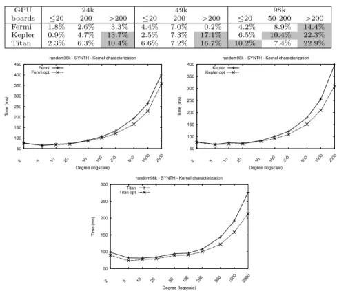
Table 4 Best performance gains for the synthetic random graphs for the used GPU boards. Gains above 10% are highlighted in grey.

GPU 24k 49k 98k

boards ≤20 200 >200 ≤20 200 >200 ≤20 50-200 >200 Fermi 1.8% 2.6% 3.3% 4.4% 7.0% 0.2% 4.2% 8.9% 14.4% Kepler 0.9% 4.7% 13.7% 2.5% 7.3% 17.1% 6.5% 10.4% 22.3% Titan 2.3% 6.3% 10.4% 6.6% 7.2% 16.7% 10.2% 7.4% 22.9%

50 100 150 200 250 300 350 400 450

2 5 10 20 50 100 200 500 1000 2000

Time (ms)

Degree (logscale) random98k - SYNTH - Kernel characterization

Fermi Fermi opt

50 100 150 200 250 300 350 400

2 5 10 20 50 100 200 500 1000 2000

Time (ms)

Kepler Kepler opt

50 100 150 200 250 300

2 5 10 20 50 100 200 500 1000 2000

Time (ms)

Titan Titan opt

Fig. 5 Scenario B: Execution times of GPU Crauser implementation and its optimized

version for the synthetic random graphs using Fermi, Kepler, and Titan boards.

up to 32.20×compared to the GPU Mart´ın. For the Dimacs set, the highest speedups obtained are up to 45.38× and up to 130.25× against the CPU Crauser and the GPU Mart´ın approaches, respectively.

B. GPU Crauser optimization

Figure 5 shows that the use of the kernel characterization techniques cited to choose optimized configuration parameters (thread-block size and L1 cache configuration) leads to significant percentages of performance improvements. The most significant are 14.39% for Fermi, 22.28% for Kepler, and 22.93% for Titan (see Table 4). Note that, for the particular scenario of graph 49k with degree greater than 200, there is hardly any improvement because the proper values selected coincide with those used in the default configuration. The performance gains obtained for real-world graphs are up to 9% for walshaw graphs and almost 6% for social networks and kronecker graphs (see Fig. 6).

(15)

0 50 100 150 200 250 300 350 400

1114316386 45087 78136 99617 143437

Time (ms)

Nodes

Walshaw - DIMACS - Kernel characterization

Fermi Fermi opt Kepler Kepler opt Titan Titan opt 0 500 1000 1500 2000 2500 3000 3500

65536131072262144 524288 1048576 2097152

Time (ms)

Nodes

Kronecker - DIMACS - Kernel characterization

Fermi Fermi opt Kepler Kepler opt Titan Titan opt

Fig. 6 Scenario B: Execution times of GPU Crauser implementation and its optimized

version for social networks and kronecker graphs using Fermi, Kepler and Titan boards.

20 40 60 80 100 120 140 160 180

2 20 200 1000 2000

Time (ms)

Degree (logscale) random24k - SYNTH - GPU architecture comparative

Fermi Kepler Titan 0 50 100 150 200 250

2 20 200 1000 2000

Time (ms)

Fermi Kepler Titan 50 100 150 200 250 300 350 400

2 5 10 20 50 100 200 500 1000 2000

Time (ms)

Fermi Kepler Titan

Fig. 7 Scenario C: Comparison of CUDA architectures using the optimized GPU Crauser

implementation for synthetic random graphs executed on the considered boards.

improvements, also using the last Kepler architecture GK110, not tested on the original work.

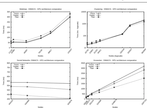
C. NVIDIA platform comparison

(16)

0 50 100 150 200 250 300 350

1114316386 45087 78136 99617 143437

Time (ms)

Nodes

Walshaw - DIMACS - GPU architecture comparative

Fermi Kepler Titan

10 100 1000 10000

16726 22963 31163 40421 192244 325557 862664

Nodes (logscale)

Clustering - DIMACS - GPU architecture comparative

Fermi Kepler Titan

400 450 500 550 600 650 700 750 800

434102 540486 820878

Time (ms)

Nodes

Social Networks- DIMACS - GPU architecture comparative

Fermi Kepler Titan

0 500 1000 1500 2000 2500 3000 3500

65536131072262144 524288 1048576 2097152

Time (ms)

Nodes

Kronecker - DIMACS - GPU architecture comparative

Fermi Kepler Titan

Fig. 8 Scenario C: Comparison of CUDA architectures using the optimized GPU Crauser

implementation for Dimacs graphs executed on the considered boards.

experimental study. Finally, for more dense graphs, the Titan board reaches the best performance with a gain of up to 40.53%, as compared with Fermi. This behavior also appears for the other graphs, but the meeting point between both architectures decreases as the graph size increases.

This occurs because the Fermi board has a lower number of cores (480) than the other tested boards (1 536 for Kepler and 2 880 for Titan), but a higher clock rate (1.40 Ghz against 1.05 and 0.89. . .0.98 Ghz). Thus, for graphs with a low degree, where the level of parallelism is lower, it is better to use a higher clock-rate GPU with fewer cores instead of a slower one with more processing units. On the other hand, having higher degrees, there are more threads performing useful relaxing operations. Therefore, for graphs with high degree and high size, it is better to use a GPU with many more cores to exploit higher levels of parallelism.

For the input set provided by Dimacs and the flickr graph, the GPU boards have returned analogous results to those of the synthetic random graphs, where Fermi is the fastest one for low size and low degree graph instances, and later Titan as these features increase (see Fig. 8).

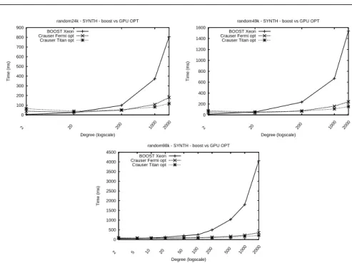
D. Boost library vs GPU Crauser optimized

(17)

0 100 200 300 400 500 600 700 800 900

2 20 200 1000 2000

Time (ms)

Degree (logscale) random24k - SYNTH - boost vs GPU OPT

BOOST Xeon Crauser Fermi opt Crauser Titan opt

0 200 400 600 800 1000 1200 1400 1600

2 20 200 1000 2000

Time (ms)

0 500 1000 1500 2000 2500 3000 3500 4000 4500

2 5 10 20 50 100 200 500 1000 2000

Time (ms)

Fig. 9 Scenario D: Execution times of the optimized GPU Crauser implementation,

ex-ecuted on Fermi and Titan boards, versus the optimized sequential Dijkstra’s algorithm included in the Boost Graph Library, for synthetic random graphs.

0 50 100 150 200 250 300 350

1114316386 45087 78136 99617 143437

Time (ms)

Nodes Walshaw - DIMACS - boost vs GPU OPT

1 10 100 1000 10000

16726 22963 31163 40421 192244 325557 862664

Nodes (logscale) Clustering - DIMACS - boost vs GPU OPT

400 600 800 1000 1200 1400 1600

434102 540486 820878

Time (ms)

Nodes

Social Networks- DIMACS - boost vs GPU OPT

0 1000 2000 3000 4000 5000 6000 7000 8000 9000 10000

65536131072262144 524288 1048576 2097152

Time (ms)

Nodes Kronecker - DIMACS - boost vs GPU OPT

Fig. 10 Scenario D: Execution times of the optimized GPU Crauser implementation,

(18)

low level of parallelism associated. Thus, the sequential algorithms work better than the parallel GPU implementation (6.8×faster than Fermi). However, as the complexity of the graph, in terms of size and degree, starts to increase, also augmenting the level of parallelism, the execution times of the Boost library start to grow linearly, whereas the execution times of the GPU solution do so logarithmically. The greater the size of the graph, the earlier the performance of the GPU solution surpasses the sequential one: (1) deg200 for the 24k-size scenarios, with a speedup of 2.13×; (2) deg20 for the 49k-size scenarios with a speedup of 1.28×; and (3) deg10 for the 98k-size scenarios with a speedup of 1.24×. Finally, our GPU solution reaches a total speedup of 6.9×, 10×, and 19×for the synthetic random graphs with degree 2 000 and 24k, 49k, and 98k nodes, respectively, using the Titan board.

Figure 10 shows the same experimental scenario for real-world graphs, where similar conclusions can be obtained. The Boost library implementation performs well in the walshaw graph family, with speedups of up to 13.09× vs our optimized version. However, our GPU approach starts to get closer to it in the clustering graphs, and finally offers a better performance than the Boost version in social-network and kronecker graphs (with speedups of up to 4.76×), while requiring lower quantities of memory.

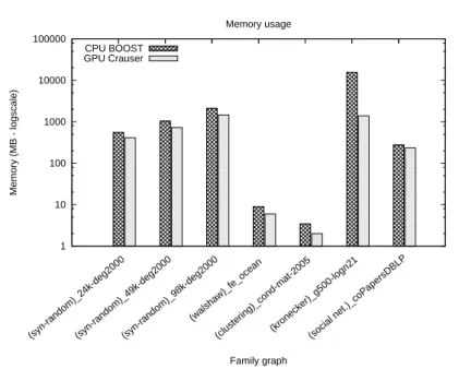
The memory usage of each approach, displayed in Fig. 11, is different due to the nature of each algorithm. The sequential implementation uses relaxed heaps as queue data structure to store the reached nodes. When there are many connections per node in a graph, the space usually needed by this queue increases exponentially, making the computation impractical for cases with big sizes and non-low fan-out degree. In comparison, our GPU solution only has three additional vectors, in addition to the data structures to store the graph, and they do not increase their space along the execution (see Sect. 3.2), leading to a consumption of up to 11.25×less memory space (kronecker g500-logn21 graph).

6 Conclusions and Future Work

We have adapted the Crauseret al.SSSP algorithm to exploit GPU architec-tures. We have compared our GPU-based approach with its sequential version for CPUs, and with the most relevant GPU implementations presented in [6]. We have obtained significant speedups for all kinds of graphs compared with the previous approaches tested, up to 45× and 130× respectively. We have also compared an optimized version of our GPU solution with the optimized sequential implementation of the Boost library [5].

(19)

1 10 100 1000 10000 100000

(syn-random)_24k-deg2000(syn-random)_49k-deg2000(syn-random)_98k-deg2000 (walshaw)_fe_ocean(clustering)_cond-mat-2005 (kronecker)_g500-logn21(social net.)_coPapersDBLP

Memory (MB - logscale)

Family graph Memory usage

CPU BOOST GPU Crauser

Fig. 11 Scenario D: Memory usage, in MB with logarithmic scale, of Boost library and

GPU Crauser for a particular graph of the different graph families.

the same reason. However, our approach runs faster when the size and degree increases, obtaining a speedup of up to 19×for some graph families.

Additionally, we have successfully tested the optimization process in our GPU solution, using the values obtained through the kernel characterization criteria from [17] for the CUDA running parameters (thread-block size and L1 cache configuration). This optimized version obtains performance benefits for all tested input sets of up to 22.43% as compared to the non-optimized version. Most recent GPU architectures contain higher amounts of single processors at the cost of reducing clock frequency, in order to take advantage of the huge parallelism levels of the applications. However, as can be seen in our experi-mental results, there is a threshold, related to the low application parallelism level, where previous CUDA architectures, working with higher clock frequen-cies, obtain better execution times. Therefore, the faster architecture in this application domain is not always the most modern one, but depends on the features of the corresponding input set.

We have detected that there is a high amount of dummy instructions exe-cuted in therelax kernel, up to 96%. The application of methods that try to avoid this dummy computation may insert more computational load than the overhead we want to avoid. Besides this, as we have already shown, although this kernel contains divergent branches, they hardly affect its performance.

(20)

Acknowledgments

This research has been partially supported by the Ministerio de Econom´ıa y Competitividad (Spain) and ERDF program of the European Union: CAPAP-H5 network (TIN2014-53522-REDT), MOGECOPP project (TIN2011-25639); Junta de Castilla y Le´on (Spain): ATLAS project (VA172A12-2); and the COST Program Action IC1305: NESUS.

References

1. H. Bast, D. Delling, A. Goldberg, M. Muller-Hannemann, T. Pajor, P. Sanders, D. Wag-ner, and R. Werneck, “Route Planning in Transportation Networks,” Microsoft Re-search, Tech. Rep. MSR-TR-2014-4, 2014.

2. D. Papadias, J. Zhang, N. Mamoulis, and Y. Tao, “Query processing in spatial network databases,” inVLDB’03. Berlin: VLDB Endowment, 2003, pp. 802–813.

3. C. Barrett, R. Jacob, and M. Marathe, “Formal-language-constrained path problems,” vol. 30, pp. 809–837, 2000.

4. E. W. Dijkstra, “A note on two problems in connexion with graphs,”Numerische Math-ematik, vol. 1, pp. 269–271, 1959.

5. J. G. Siek, L.-Q. Lee, and A. Lumsdaine,The Boost Graph Library: User Guide and Reference Manual. Boston, MA, USA: Addison-Wesley Longman Publishing Co., 2002. 6. P. Mart´ın, R. Torres, and A. Gavilanes, “CUDA Solutions for the SSSP Problem,” in

Computational Science – ICCS 2009, ser. LNCS, G. Allen, J. Nabrzyski, E. Seidel, G. van Albada, J. Dongarra, and P. Sloot, Eds. Springer, 2009, vol. 5544, pp. 904–913. 7. P. Harish, V. Vineet, and P. J. Narayanan, “Large Graph Algorithms for Massively Multithreaded Architectures,” Centre for Visual Information Technology, International Institute of IT, Hyderabad, India, Tech. Rep. IIIT/TR/2009/74, Feb. 2009.

8. D. B. Kirk and W. W. Hwu,Programming Massively Parallel Processors: A Hands-on Approach. Morgan Kaufmann, Feb. 2010.

9. A. Crauser, K. Mehlhorn, U. Meyer, and P. Sanders, “A parallelization of Dijkstra’s shortest path algorithm,” inMathematical Foundations of Compt. Science 1998, ser. LNCS, L. Brim, J. Gruska, and J. Zlatuˇska, Eds. Springer, 1998, vol. 1450, pp. 722–731. 10. T. H. Cormen, C. Stein, R. L. Rivest, and C. E. Leiserson,Introduction to Algorithms,

2nd ed. Burr Ridge, Il 60521: McGraw-Hill Higher Education, 2001.

11. M. L. Fredman and R. E. Tarjan, “Fibonacci heaps and their uses in improved network optimization algorithms,”J. ACM, vol. 34, pp. 596–615, July 1987.

12. D. P. Singh and N. Khare, “Article: A Study of Different Parallel Implementations of Single Source Shortest Path Algorithms,”Int. Journal of Computer Applications, vol. 54, no. 10, pp. 26–30, September 2012.

13. M. Papaefthymiou and J. Rodrigue, Implementing parallel shortest-paths algorithms, ser. DIMACS Series in Discrete Mathematics and Theoretical Computer Science. Prov-idence: American Mathematical Society, 1994, vol. 30, pp. 59–68.

14. U. Meyer and P. Sanders, “∆-Stepping: a parallelizable shortest path algorithm,”

Journal of Algorithms, vol. 49, no. 1, pp. 114–152, 2003. [Online]. Available: http://www.sciencedirect.com/science/article/pii/S0196677403000762

15. A. Davidson, S. Baxter, M. Garland, and J. Owens, “Work-Efficient Parallel GPU Meth-ods for Single-Source Shortest Paths,” inParallel and Distributed Processing Sympo-sium, 2014 IEEE 28th International, May 2014, pp. 349–359.

16. M. Harris, Optimizing Parallel Reduction in CUDA, devel-oper.download.nvidia.com/assets/cuda/files/reduction.pdf, nVidia, 2008.

17. H. Ortega, Y. Torres, A. Gonzalez-Escribano, and D. R. Llanos, “Optimizing an APSP Implementation for NVIDIA GPUs Using Kernel Characterization Criteria,”J. Super-computing, pp. 1–13, 2014.

18. S. Nobari, X. Lu, P. Karras, and S. Bressan, “Fast random graph generation,” in

Proc. of the 14th International Conference on Extending Database Technology, ser. EDBT/ICDT ’11. New York, NY, USA: ACM, 2011, pp. 331–342.

19. “DIMACS implementation challenge,” 2012. [Online]. Available: http://www.cise.ufl.edu/research/sparse/dimacs10