TítuloA simple procedure to select a model for mass discrimination correction in isotope dilution inductively coupled plasma mass spectrometry

(1)

A simple procedure to select a model for mass

discrimination correction in isotope dilution

inductively coupled plasma mass spectrometry

J. Ter´an-Baamonde, J. M. Andrade,* R. M. Soto-Ferreiro, A. Carlosena and D. Prada

A fast, simple and straightforward procedure to decide on the best model to calculate the mass discrimination factor in Isotope Dilution Inductively Coupled Plasma Mass Spectrometry (ID-ICP-MS) is proposed. It is based on the study of the residuals of the different models that are proposed commonly, viz., the linear, the exponential, the power and Russell's models. However, it can be generalized to evaluate any model proposed to linearize the relationship between the theoretical/measured isotope ratios and the mass. The procedure does not involve laboratory extra work, it is rooted on basic statistics associated with the least squaresfit, and can be applied easily by the analysts so that decision making is fast and reliable. The procedure was exemplified with four different examples where Cd, Cr, Nd and Sm were determined by ID-ICP-MS.

Introduction

Isotope dilution inductively coupled plasma mass spectrometry (ID-ICP-MS) has become a work horse technique to quantify metals at trace and ultra trace levels, study their species and, more recently, determine proteins (using either inspecic and species-specic methods).1–3 _{This can be explained, amongst} other considerations, because isotope dilution mass spec-trometry (ID-MS) was recognized as a denite primary method, meeting the highest metrological standards, by the ‘Comité Consultative pour la Quantité de Matière (CCQM)’ and so its results are directly traceable to SI units.4

Further, in most ID-MS applications the typical working calibration graphs based on the use of calibration solutions of diﬀerent quantities of the analyte may be avoided. This saves costly instrument time and makes ID-MS applications much more robust than conventional methodologies so less-careful sample preparation is required. Also, ID-MS procedures are more accurate than conventional methodologies, so that fewer quality-control failures are to be expected.5

However, adequate training of laboratory staffis required as ID-ICP-MS needs a careful and laborious optimization in order to look for the best measuring conditions that yield a reliable and traceable working chain. A relevant issue here is to recall that a mass discrimination occurs in ICP-MS when ions of different mass are transmitted through the spec-trometer, leading to different efficiencies in the transport of ions which results in non-uniform sensitivity across the mass range and inaccurate isotope ratio measurements.6

Following, ICP-MS devices may yield biased isotope amount ratios7_{and, therefore, mass discrimination must be corrected} for using a correction factor, termed mass discrimination factor,K(it is oen presented, simply, as the‘mass bias’or ‘mass bias factor’, or‘mass bias factor per unit mass’). This is dened as the quotient between the true and the measured mass ratios for a pair of given isotopes and so it underlines that the instrumental system may yield a systematic error regarding the correct mass ratio.8–10

It is worth noting thatKis dened and determined locally for a specic isotope pair. This raises a further potential diﬃculty asKmay incorporate contributions from unsuspected spectral interferences which could vary from sample to sample and, thus, make it unrepresentative of the bias obtained for adjacent masses.6

In general, two approaches exist to correct for mass discrimination, measured by K.11 _{First, external} stand-ardisation, where the isotope ratio of interest is measured in a standard solution of exactly known composition of the analyte to be analyzed, and the experimental bias is used to correct the same ratio in the unknown sample. This allows the mass discrimination factor to be measured at the same masses as the analyte, and approximately at the same abundances. Second, internal standardisation determines the mass discrimination factor of the isotope ratio of interest in the unknown sample solution by means of either a known isotope ratio of an element added to the sample for that purpose, or using a pair of invariant isotopes of the analyte element.6 Another relevant issue is that K can dri throughout the experiment time and, thus, it must be determined periodi-cally. A standard bracketing sequence is adopted usually, yielding low throughput.10

Dept. Qu´ımica Anal´ıtica, Universidade da Coru˜na, Campus da Zapateira, s/n, E-15071, A Coruna, Spain. E-mail: andrade@udc.es; Fax: +34-981167065˜

Cite this:J. Anal. At. Spectrom., 2015,

30, 1197

Received 12th December 2014 Accepted 8th January 2015

DOI: 10.1039/c4ja00475b

www.rsc.org/jaas

TECHNICAL NOTE

Open Access Article. Published on 21 January 2015. Downloaded on 20/10/2015 17:02:43.

This article is licensed under a

Creative Commons Attribution-NonCommercial 3.0 Unported Licence.

View Article Online

(2)

The relative magnitude of mass discrimination can be ascertained using multielemental molar-response curves by which the response observed in the detector is measured as a function of the ion transmission eﬃciency through the system.5 In general, these curves have to span through a range of mass/ charge values, and are complex and depend on the instrument at hand. To make them useful it is necessary to model them functionally. All models calculate a corrected isotope ratio (Rcorr) from an experimentally measured one (Rexp), the absolute masses of the isotopes (mi and mj), or the mass diﬀerence between the isotopes (DM), andK(the mass bias factor, which must be determined empirically).

Three functions are of general use; viz. the linear, the exponential and the power ones. They were critiziced somehow by Ingleet al.6_{because they predicted that the bias} was dependent on the mass diﬀerence and not on the abso-lute mass. Besides, they have a common origin and the former two may be considered as approximations to the power model.6,12_{Further, in these functions}_K_{should be considered} as the mass bias per unit mass and it is assumed to be constant across the mass range and proportional, which is not totally correct.6 _{This explains why Russell's model became} popular because it avoids these problems as it uses the mass of the two isotopes.

Even though the models might yield similar mass bias factors, inaccuracy may arise from the use of an inappropriate one.13_{Accordingly, the selection of the most suitable functional} model is not trivial. Indeed, calculating the mass bias factor is far from a standardized procedure and is demonstrated by the existence of several approaches. Some can be mentioned here (a complete review is out of the scope of this technical note).Kwas determined as the ratio between the theoretical, or true, isotope ratio and the same ratio measured experimentally.8_Then,_K_can be applied using either a bracketing approach or a mathemat-ical model.4,6,14 _{The use of several internal reference isotope} pairs was compared against the classical approaches mentioned above.11_{This implied the use of a polynomial function and the} so-called ‘common analyte internal standardization’. The results emphasized the importance of a proper mass discrimi-nation correction (along with the need for a selection of an adequate internal standard).

To complicate things further, the reasons why a model was selected have not always been claried.15–17

Following, this paper aims at presenting a fast and simple procedure to select the best model to calculate the mass discrimination factor in ID-ICP-MS. The key idea is to study and

compare the residuals of the diﬀerent linearized models. Here we will consider the most common ones;viz., the exponential, the linear, the power and Russell's models, although the procedure can be generalized to any other. Four examples will be considered where Cd, Cr, Sm and Nd were determined.

Evaluation of the mass bias factor per unit mass

From a pragmatic viewpoint, the most convenient way to model the instrumental mass discrimination is to relate a suite of theoretical isotope ratios (Rtheo) to their corresponding empir-ical values (Rexp), calculateKand, then, use it (along withRexp) to calculate a corrected ratio (Rcorr) for the unknown. In general,K is involved in an algebraic equation describing a curve but it can be calculated straightforwardly whenever a linear model is used instead.6,8

As discussed in the previous section, the empirical rela-tionship betweenRtheo,Rexpand the two isotope masses can be described in diﬀerent ways, among which four stand out in the literature: the linear (straight line), the exponential, the power and Russell's models. They are depicted in the second column of Table 1. As their direct use is not trivial, the common practice is to linearize them to get simpler and more straightforward equations (see the third column of Table 1). To select the best model for a particular problem it was proposed tot the four linearized models and to study the straight lines obtained by plotting theRtheo/Rexpratio (or a logarithmic form) against the mass diﬀerence (or logarithm of the masses, in Russell's model).5 _{However, this approach is subjective and prone to} errors because the signicance of those plots is not immediate and a sound decision making is not possible.

Fortunately, basic statistics associated with the straight line (orrst-order) least squarest yield very simple and reliable criteria to judge on the adequacy of each linearized model.18–20 Note that the expression ‘straight line t’ will be used throughout the text to denote that the models are converted to a straight line function. The term‘lineart’and the like are not of suﬃcient quality to assure the traceability of the calculations because, aer all, any mathematical relationship is ‘a line’. Analogously, the term‘linearization’is used to denote an alge-braic transformation from a (usually) complex mathematical expression to a straight line equation, whose parameters are of interest (here, the slopeK).

Although the conceptual idea is really simple, it is worth remembering some basic statistics. More details and extensive explanations can be found in the references given herein.

Table 1 Models to determine the mass discrimination factor (K) in ID-ICP-MS.Rcorris the corrected isotope ratio,Rexpis the measured isotope

ratio,Rtheois the theoretical isotope ratio,miandmjare the absolute masses of the selected isotopes andDMis the mass diﬀerence between

them

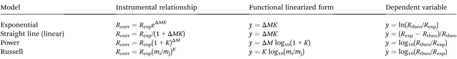
Model Instrumental relationship Functional linearized form Dependent variable

Exponential Rcorr¼RexpeDMK y¼DMK y¼ln(Rtheo/Rexp)

Straight line (linear) Rcorr¼Rexp/(1 +DMK) y¼DMK y¼(RexpRtheo)/Rtheo Power Rcorr¼Rexp(1 +K)DM y¼DMlog10(1 +K) y¼log10(Rtheo/Rexp) Russell Rcorr¼Rexp(mi/mj)K y¼Klog10(mi/mj) y¼log10(Rtheo/Rexp)

(3)

Review of some concepts associated with the straight linet

In a typical model, two variables are related asy¼f(x) +3, where

f(x) is a mathematical function that relatesytox(it is a common practice to select a straight line function but other possibilities exist, and the choice is under the analyst's responsibility based on his/her experience and/or experimental data). Note that the model is a mere working hypothesis, which must be modied if the experimental data are against it. Finally,3 is the random error, or information not modelled by the calibration function, which is associated with the variable response and denotes how closely the model resembles the measured signals. It is reasonable to accept that the smaller the random errors are, the better the model is. Therefore, how can wet the best model through a swarm of points? A quite intuitive solution is to look for a model that adheres as much as possible to each and every experimental point so that it minimizes the average difference between the experimental signals and those predicted by the model. Hence, the common criterion by which the sum of the squared differences between the measured signal (yexp) and that predicted by the model (ypred) is minimal was accepted as a natural tting criterion.18–20_{The di}_ff_{erences (}_y

pred yexp) are referred to as‘residuals’. This is the (ordinary) least squares criterion (OLS or LS). Despite its widespread and ubiquitous usage the OLS criterion has three basic mathematical assump-tions that are less broadly known:18–22

(i) the experimental errors occur only in the direction of the signal to be measured,y.

(ii) The errors in they-direction are normally distributed. This means that the resulting errors associated with the analytical signals should follow a normal distribution.

(iii) The errors in they-direction are independent and of the same magnitude regardless of the xvalues. This property is referred to as ‘homoscedasticity’ (the opposite situation is called‘heteroscedasticity’). Its presence simplies the calcula-tions and gives rise to the usual unweighted least-squares line. Statements (ii) and (iii) above constitute two cornerstones to assure whether a modelt is acceptable. Since the OLS criterion is a universal procedure tot functions, it does not guarantee by itself that the model under scrutiny is correct. In order to accept it, we must assess that these two requisites hold on. There are diﬀerent statistical tests to evaluate the models but most of them should not be used due to the usual low number of data points employed tot the model23_{(this will be considered later).} Therefore, a suitable alternative consists of a graphical visuali-zation and evaluation of the residuals associated with our (temptative) model.

Homoscedasticity of thet must be assured and, fortunately, can be visualized easily. First, the absence of outlying points must be checked as they may strongly bias any model in different ways,24_{see Fig. 1a and b for a general, conceptual idea} on how strongly an outlier will inuence the regression. In general, outliers situated in extreme positions affect more thet (rotational effects).22_{Check that all points do follow a unique} trend; in case a point behaves anomalously, consider rejecting it and recalculating the model. Sometimes, decisions are not immediate and plotting the residuals will help. This can be

done straightforwardly in any spreadsheet, less than a minute, and it may yield enormous benets. Any data point with a too high residual is suspicious (more formally, a point whose standardized residual is around 3, or higher, should be considered as an outlier23_{). Next, check for the absence of visual} trends in the residuals (Fig. 1c and d). In particular, parabolic trends are frequent (Fig. 1d) and they mean that a straight line does nott the experimental data properly. If a clear trend is not visualized, all residuals are more or less randomly distributed, and are of the same magnitude (Fig. 1c), it can be reasonably assured that they are normally distributed and that they have common variance (another requisite of the OLS methodology).20 Normality can be studied more formally using statistical tests, as those described in the next section, where more details are presented.

It may surprise that so much emphasis is put on graphical decision-making but this can be explained quoting NIST: ‘Numerical methods for model validation are useful, but usually to a lesser degree than graphical methods. The latter have an advantage [.] because they readily illustrate a broad range of complex aspects of the relationship between the model and the data’.25

Experimental

Datasets

Four case studies will exemplify the working methodology proposed here. Two of them deal with the determination of Sm and Nd and were used as tutorials in a recent textbook.5_They present a situation where the replicates of the experimental ratios are not considered explicitly to set the model. The other two examples are about determining Cd and Cr by ID-ICP-MS, using a quadrupole analyzer equipped with a kinetic energy discrimination cell. They correspond to an ongoing study in our laboratory to measure some environmentally relevant metals in Fig. 1 Eﬀect on the regression lines calculated by the ordinary least squares criterion when outliers are present in the dataset (the rota-tional and translarota-tional denominations stem from ref. 24) and a graphical example of homoscedasticity (c) and heteroscedasticity (d) in the residuals.

(4)

sediments. Replicates of the mass isotopes are presented and, therefore, will be applied to illustrate the use of the lack-of-t test (LOF). In addition, Cr was selected because of the low number of isotopes and their low mass (compared to the other elements in the present work).

The experimental isotope ratios were obtained from measurements carried out on Cd and Cr standard solutions of natural isotope composition for ICP analysis (Sigma Aldrich) whose theoretical isotope abundances were obtained from IUPAC.26_{Table 2 shows the compiled experimental results.}

Working methodology

In the following, the diﬀerent candidate models will be considered in their functional linearized straight line forms and the unweighted OLSt obtained for each one. Therst step in selecting a model is to inspect visually the residuals (potential outliers, relative magnitudes of the residuals and the absence of clear trends) and to study the statistics associated with the regression line (the standard error of the t, or residual

standard deviation, Sy/x). A careful inspection and a bit of experience are usually enough to make sound decisions, as it will be shown next.

Note that as a referee pointed out, the units ofSy/xdepend on the particular transformation undergone by the data. Hence, to compare them it is necessary to get rid of the scales. A natural way would be to divideSy/xby an average value (like the classical relative standard deviation, RSD). However, this is not possible here because the average value of the residuals is zero. To circumvent this problem, the average absolute error (i.e., the average of the absolute values of the residuals), yres, is proposed here to get a sort of‘relative standard deviation of the t’, RSDF as: RSDF ¼ 100*((Sy/x)/yres). As classical RSD, it shows the extent of the variability of the residuals in relation to the average value (of the absolute residuals).

In addition, two traditional scale-independent statistics were also considered: the coeﬃcient of determination (R2) and the lack-of-t test (which must be derived from an Analysis of Variance–ANOVA–study when replicates are available).27_Both are used to evaluate the adequacy of the model to the Table 2 Original data for the four case studies considered here. The isotopes selected for each element are shown under the heading‘Isotopes’, along with their theoretical (derived from IUPAC26_{) and experimentally measured ratios. The mass di}ﬀ_{erence is denoted as}DMa,b

Isotopes

Theoretical ratio

Experimental

ratio DM Isotopes Theoretical ratio

Experimental

ratio DM Isotopes

Theoretical ratio

Experimental ratio DM

Case study 1: Cd

106/114 0.043508528 0.031349113 8 111/114 0.445527323 0.391757742 3 113/114 0.425339367 0.406410177 1

0.031121068 8 0.391053577 3 0.405081916 1

0.030958661 8 0.394968971 3 0.406683127 1

0.030647223 8 0.392116797 3 0.406479036 1

0.030951996 8 0.393185914 3 0.405911499 1

108/114 0.030978072 0.023971763 6 112/114 0.839888618 0.772383915 2 116/114 0.260703098 0.279916302 2

0.023763753 6 0.768285734 2 0.278555226 2

0.0247017* 6 0.775911501 2 0.279184221 2

0.024381751 6 0.774078028 2 0.281141181 2

0.02392011 6 0.772314239 2 0.279164297 2

110/114 0.434737208 0.365326652 4 0.365379831 4 0.370625246 4 0.36543465 4 0.366794537 4

Case study 2: Cr

50/52 0.051456543 0.04146233 2 53/52 0.114016237 0.126390065 1 54/52 0.028414518 0.035143948 2

0.039952749* 2 0.125910941 1 0.03487478 2

0.041939234 2 0.125490294 1 0.034398109 2

0.042557359 2 0.126713427 1 0.036049048 2

0.042027005 2 0.127015489 1 0.035308014 2

0.042005136 2 0.125975986 1 0.03475144 2

0.041460437 2 0.126565896 1 0.035736555 2

0.040932561 2 0.125553057 1 0.034422643 2

Case study 3: Nd (**) Case study 4: Sm (**)

142/146 1.57961487 1.491953 4 144/147 0.2048032 0.197872 3

143/146 0.70824364 0.679507 3 148/147 0.74983322 0.758822 1

144/146 1.38449008 1.345698 2 149/147 0.92194797 0.943961 2

145/146 0.48245971 0.475716 1 150/147 0.49232822 0.510151 3

148/146 0.33486532 0.34442 2 152/147 1.78452302 1.891842 5

150/146 0.32800047 0.346675 4 154/147 1.51767845 1.647119 7

a₍_*_{) Outliers excluded from the studies.}b₍_**_{) Case studies 3 and 4 stem from ref. 5.}

(5)

experimental data. In simple linear regression, the former equals the squared correlation coeﬃcient (given in percentage), but this cannot be generalized to other situations and it is a rough approach to evaluate goodness-of-t. The lack-of-t test is an F-test which determines whether the residual information can be associated with the experimental random errors or with ‘something’else (i.e., the model has not been able to capture all the relevant variance in the data points and therefore causes a ‘lack-of-t’). Though both tests can be used to compare among diﬀerent regression models, they should be used in conjunction with the residual plots because they are not powerful enough to assure by themselves that the model is suitable28,29 _{(a typical} problem is that even curvilinear models can exhibit very good gures in both parameters).

Then, statistical tests can be applied to check the normality of the residuals. A normal probability curve (avail-able in most common soware) will also simplify decision making. However, as mentioned above, usual calibrations in analytical chemistry do not imply many experimental points due to work, time and resources constraints. As a conse-quence, it is diﬃcult (sometimes impossible) to rely on sound statistics for decision making due to the low power of the tests (very few degrees of freedom). Non parametric statistics might constitute a powerful alternative but, again, they are not good enough when very few data are available. A clear example here was the impossible application of the non parametric Wald– Wolfowitz's runs test (to check for a random distribution of the residuals) to the Nd and Sm examples due to a lack of tabulated values for such a small number of runs (because of the few data points).

Here, the standardized Kurtosis and Skewness were calcu-lated as a way to describe whether the distribution of the residuals is symmetric and without tails. Then, the non para-metric sign test and the Wilcoxon's signed rank test were used

to check whether the residuals are distributed randomly. Finally, the Kolmogorov–Smirnov's and the Shapiro–Wilk's tests (the latter is more powerful than the Kolmogorov–Smirnov's one when few data are available) were used to check whether the distribution of the experimental residuals is compatible with a Gaussian one.22

Fig. 2 shows the working procedure conceptually.

Soware

The statistical studies were performed using Excel® and Stat-graphics (StatPoint Technologies, Inc., Warrenton, VA, USA).

Results and discussion

Case study 1 and 2: selection of the model when determining Cd and Cr

Table 3 shows the results of several statistical tests calculated on the residuals of the diﬀerent models whereas Fig. 3 and 4 depict the residuals associated with each model and each example, along with the standard error of the calibration (Sy/x), the rela-tive standard deviation of the t (RSDF), the coeﬃcient of determination (R2) and the lack-of-t test (LOF).

With respect to Cd, a replicate was rejected because it had an outlying behaviour throughout the studies (see Table 2). The linear (straight-line)t presents a rather clear parabolic pattern (Fig. 3) and, so, it has to be discarded. This model shows also a signicant lack-of-t (95% condence) and, accordingly, it is not suitable for our purposes. The other models do not exhibit a clear trend and, thus, are considered further. The exponential and power models (whose behaviour is almost equal) present a borderline lack-of-t (LOF). Although, strictly speaking, the test is not signicant as the experimentalp-value associated with theFtest is too close to the critical one (0.05, 95% condence). Finally, the residuals for Russell's method do not have a denite pattern, the LOF test is clearly not signicant, the RSDF is comparable to the other models and theR2statistic is marginally better. There-fore, the latter model should be selected.

This conclusion was assured by studying the residuals of the models deeper and calculating the statistics mentioned above. Table 3 reveals that no model had either a skewed distribution or a tailed shape (standardized skewness and kurtosis lower than2). Thus, these statistics do not help in deciding on the best model.

The null hypotheses of the sign test and of the Wilcoxon's signed rank test (in both cases, H0: the data derive from a population with a median value of zero) cannot be rejected for any model, hereby revealing that the sets of residuals are compatible with a symmetric distribution whose median is zero. However, this does not guarantee that they are normally distributed.22

The other tests are intended to check whether the distribu-tion of the residuals is Gaussian (H0: the distribution of resid-uals follows a normal distribution); namely, the Shapiro–Wilk's and the Kolmogorov–Smirnov's tests. In Table 3 no rejection can be made so all models are compatible with the normal Fig. 2 Conceptual description of the approach proposed to select the

most suitable model to calculate the mass discrimination factor,K.

(6)

distribution of the residuals. The other tests yielded the same conclusion (but for a borderline situation of the straight line model when the Shapiro–Wilk's test was used).

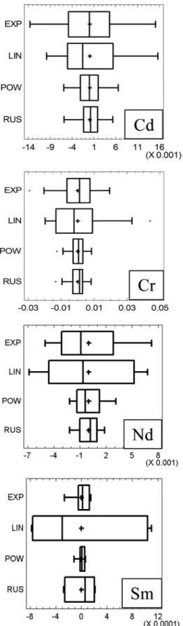
Finally, Russell's method led to the lowest dispersion of the residuals (Fig. 5). Therefore, there is not additional evidence against the selection of Russell's model for Cd.

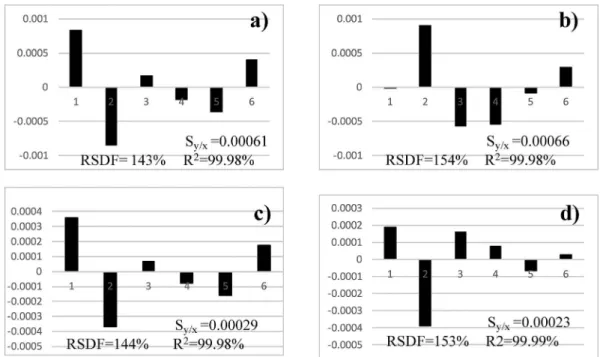
Fig. 3 Case study 1 (Cd): statistics associated with the calibration and graphical representation of the residuals. Models to calculate theKfactor: (a) exponential, (b) straight-line, (c) power, and (d) Russell.

Table 3 Statistics associated with the residuals of the models developed to calculate the mass bias factor in each case study. See text for details

Case study Exponential Straight line Power Russell

Cd Skewness 0.14 1.41 0.14 0.48

Kurtosis 0.01 0.46 0.01 0.44

Sign test p-value¼1.00 p-value¼0.39 p-value¼1.00 p-value¼0.61 Wilcoxon's test p-value¼1.00 p-value¼0.78 p-value¼1.00 p-value¼0.76 Shapiro–Wilk`s test p-value¼0.99 p-value¼0.16 p-value¼0.99 p-value¼0.54 Kolmogorov–Smirnov`s test p-value¼0.99 p-value¼0.65 p-value¼0.99 p-value¼0.89

Cr Skewness 1.26 2.13 1.26 1.61

Kurtosis 0.53 0.80 0.53 0.57

Sign test p-value¼1.00 p-value¼0.40 p-value¼1.00 p-value¼0.40 Wilcoxon's test p-value¼0.75 p-value¼0.57 p-value¼0.75 p-value¼0.70 Shapiro–Wilk test p-value¼0.30 p-value¼0.03 p-value¼0.29 p-value¼0.21 Kolmogorov–Smirnov's test p-value¼0.93 p-value¼0.71 p-value¼0.93 p-value¼0.88

Nd Skewness 0.05 0.75 0.05 1.52

Kurtosis 0.22 0.13 0.22 1.24

Sign test p-value¼1.00 p-value¼0.68 p-value¼1.00 p-value¼0.68 Wilcoxon's test p-value_¼1.00 p-value_¼0.83 p-value_¼1.04 p-value_¼0.68 Shapiro_–Wilk test p-value_¼0.99 p-value_¼0.53 p-value_¼0.99 p-value_¼0.19 Kolmogorov_–Smirnov's test p-value_¼1.00 p-value_¼0.99 p-value_¼1.00 p-value_¼0.93

Sm Skewness 1.12 0.71 1.12 0.56

Kurtosis 0.57 0.94 0.57 0.94

Sign test p-value¼1.00 p-value¼0.68 p-value¼1.00 p-value¼0.68 Wilcoxon's test p-value¼1.00 p-value¼1.00 p-value¼1.04 p-value¼1.00 Shapiro–Wilk's test p-value¼0.34 p-value¼0.07 p-value¼0.34 p-value¼0.14 Kolmogorov–Smirnov's test p-value¼0.94 p-value¼0.75 p-value¼0.94 p-value¼0.89

(7)

With respect to Cr, the low number of isotopes yields only three diﬀerent calibration levels, which complicates decision making. However, the linear model shows a clear trend (Fig. 4) which makes it unsuitable (Fig. 2). This was conrmed by the high skewness of the residuals (Table 3), a bad normal proba-bility plot (gure not shown) and a high dispersion of its residuals (Fig. 5). Further, theR2and LOF revealed that it is the model thatts the experimental data worst. Hence, it should be discarded denitely.

The other three models performed very similar, with good statistics for the residuals (Table 3). The R2 and LOF tests were almost equal and only marginal best RSDF values were obtained for the exponential and power models. The LOF test was not signicant for any of these three models (95% condence) although it was better for the power and exponential models than for Russells' one. As the dispersion of the residuals (Fig. 5) was slightly better for the power than for the exponential method, the former was selected for Cr.

Case study 2 and 3: selection of the model when determining Nd and Sm

Analogous studies were carried out to select the best model to determineKwhen studying Nd and Sm. These examples do not include replicates for the isotope ratios and, so, the lack-of-t test cannot be calculated. Previous studies concluded that all models, but the straight-line one, may be acceptable and the

exponential method was preferred (although there was a somehow marginal best performance of Russell's method when determining Nd).5

When the residual plots were considered for Nd (Fig. 6) it was concluded that any one showed a particularly cumbersome behaviour as all models had a quite random distribution. The model with the best RSDF was the exponential one, which agreed with the conclusion obtained elsewhere, although following a more elaborate procedure.5 _The _R2 _{statistic was} almost the same for all models and it did not allow drawing sound conclusions.

The statistics associated with the residuals, Table 3, revealed that Russell's method yielded a somehow worst distribution (skewness and kurtosis, although not statisti-cally signicant), whereas the exponential and the power methods performed the best. The latter one was selected nally for Nd because of the lowest dispersion of the residuals (Fig. 5).

When Sm was considered (Fig. 7) Russell's and the straight-line methods were not acceptable as they showed a parabolic residual pattern and, therefore, the models do nott the data properly. Hence, they are discarded at therst step of Fig. 2. It is noteworthy that the approach presented here allows an immediate and clear rejection of Russell's model, which was not so simple when calculating relative errors.5_The exponen-tial and power models behave totally similar (as noticed previously)5 _{although with a marginal better RSDF for the} power method. With regards to the residual statistics (Table 3) Fig. 4 Case study 2 (Cr): statistics associated with the calibration and graphical representation of the residuals. Models to calculate theKfactor: (a) exponential, (b) straight-line, (c) power, and (d) Russell.

(8)

they reinforce the graphical conclusions. Note that it is not possible to select between the methods (once Russell's and straight-line ones were discarded) considering the statistics alone (as for most models in the previous section, the null hypotheses of the statistical tests could not be rejected and they were of little value to select a model). The power model was selected owing to the smallest scattering of the residuals (Fig. 5).

Twonal notes can be given. First, most statistics shown in Table 3 can be visualized in a common box and whiskers plot (Fig. 5). Although – strictly speaking – such a plot is not a graphical representation of the tests, the symmetry of the residuals, their distribution and the closeness of the mean and the median can be observed easily. So, for a reduced dataset (as is usually the case), it is possible to take advantage of this plot for decision making: (i) the smaller the box and the whiskers are, the lower the standard error of the regression is; (ii) the closer the mean (in the plot this is shown by a cross) and the median (the bar within the box) are, the less likely the existence of outliers will be; (iii) the more symmetrical the box and the whiskers are, the less skewed the distribution will be and, likely, the more Gaussian the distribution of the residuals will become. Second, the RSDF was always greater than 100% because it is derived from the residuals. These, in turn, follow essentially a random distribution and, therefore, their vari-ability is expected to be large when compared to the average (of the absolute values, because the arithmetic average is zero). The relevant issue here is to look for models with the lowest RSDF values.

Conclusions

It was shown that simple plots derived from the residuals of the least squarest provide a powerful, simple and rather objective criterion to decide on the suitability of a model to calculate the mass discrimination factor (K) in ID-ICP-MS. Visualization of the residuals of thet for the diﬀerent models allows deciding on the existence of both outliers and non random (typically, parabolic) patterns.

Then, the lack-of-t test (if replicates are available) will further test the adequacy of the model. In the examples studied in this paper, the classical coeﬃcient of determination (R2) and the relative standard error of thet (RSDF) were not critical to select among diﬀerent candidate models. However their calcu-lation is straightforward and it is recommended to keep them in order to gather additional information on the models. Further, a box and whiskers plot yields good clues on the symmetry (likely, on the Gaussian distribution) and scattering of the residuals, which can help selecting amongst two very similar candidate models.

It was also observed that on some occasions non parametric statistics were not conclusive enough for decision making. Thus, the graphical study of the residuals and the lack-of-t test constitute the cornerstones to diﬀerentiate among several models to calculate the mass discrimination factor and to select a suitable one.

Fig. 5 Box and Whiskers plot of the residuals for each model (Exp¼ exponential, Lin¼straight line, Pow¼power, Rus¼Russell). The cross in the middle of the box represents the average value whereas the vertical line within the box represents the median.

(9)

Acknowledgements

The Galician Government (Xunta de Galicia; Research Grant GRC2013-047, Programa de Consolidación y Estructuración de Unidades de Investigación Competitivas) is acknowledged. J.T-B. thanks the Universidade da Coruña for a Predoctoral grant. Two anonymous referees are acknowledged by their insightful comments and suggestions to improve the original manuscript.

Notes and references

1 E. Blanco Gonz´alez and A. Sanz Medel, in Liquid chromatographic techniques for trace element speciation analysis, Elemental Speciation: a new approaches for trace element analysis, ed. J. A. Caruso, K. L. Sutton and K. L. Ackley, Elsevier, Amsterdam, Netherlands, 2000.

2 J. Gómez Espina, E. Blanco González, M. Montes Bayón and A. Sanz Medel,J. Anal. At. Spectrom., 2012,27, 1949–1954. Fig. 6 Case study 3 (Nd): standard error of thefit (Sy/x) and graphical representation of the residuals. Models to calculate theKfactor: (a) exponential, (b) straight-line, (c) power, and (d) Russell.

Fig. 7 Case study 3 (Sm): standard error of theﬁt (Sy/x) and graphical representation of the residuals. Models to calculate theKfactor: (a) exponential, (b) straight-line, (c) power, and (d) Russell.

(10)

3 Y. Nuevo Ordoñez, M. Montes-Bayón, E. Blanco-González and A. Sanz-Medel,Anal. Chem., 2010,82, 2387–2394. 4 Y. Yip, H. Chu, K. Chan, K. Chan, P. Cheung and W. Sham,

Anal. Bioanal. Chem., 2006,386, 1475–1487.

5 J. I. Garc´ıa Alonso and P. Rodr´ıguez Gonz´alez, Isotope dilution mass spectrometry, Royal Society of Chemistry, Cambridge, United Kingdom, 2013.

6 C. P. Ingle, B. L. Sharp, M. S. A. Hortswood, R. R. Parrish and D. J. Lewis,J. Anal. At. Spectrom., 2003,18, 219–229. 7 J. Ruiz Encinar, J. I. Garc´ıa Alonso, A. Sanz-Medel, S. Main

and P. J. Turner,J. Anal. At. Spectrom., 2001,16, 322–326. 8 K. G. Heumann, S. M. Gallus, G. R¨adlinger and J. Vogl, J.

Anal. At. Spectrom., 1998,13, 1001–1008.

9 US Environmental Protection Agency, Method 6800: Elemental and speciated isotope dilution mass spectrometry, 2007.

10 E. Ciceri, S. Recchia, C. Dossi, L. Yang and R. E. Sturgeon,

Talanta, 2008,74, 642–647.

11 L. Yang and R. E. Sturgeon,J. Anal. At. Spectrom., 2003,18, 1452–1457.

12 J. Mejia, L. Yang, Z. Mester and R. E. Sturgeon, in Instrumental mass discrimination for isotope ratio determination with multicollector Inductively Coupled Plasma Mass Spectrometry,Isotopic Analysis. Fundamentals and Applications using ICP-MS, ed. F. Vanhaecke and P. Degryse, Wiley-VCH, Weingeim, Germany, 2012.

13 I. S. Begley and B. L. Sharp,J. Anal. At. Spectrom., 1997,12, 395–402.

14 S. Garc´ıa-Ruiz, I. Petrov, E. Vassileva and C. R. Qu´etel,Anal. Bioanal. Chem., 2011,9, 2785–2792.

15 K. E. Murphy and T. W. Vetter,Anal. Bioanal. Chem., 2013,

405, 4579–4588.

16 H. Liu, C. You, W. Cai, C. Chung, K. Huang, B. Chen and Y. Li,Analyst, 2014,139, 734–741.

17 J. Lee, E. A. Boyle, Y. Echegoyen-Sanz, J. N. Fitzsimmons, R. Zhang and R. A. Kayser,Anal. Chim. Acta, 2011,686, 93. 18 M. C. Ortiz, S. S´anchez and L. Sarabia, in Quality of analytical

measurements: univariate regression, Comprehensive Chemometrics: chemical and biochemical data analysis, ed. S. D. Brown, R. Tauler and B. Walczack, Elsevier, Amsterdam, Netherlands, 2009.

19 N. R. Draper and H. Smith,Applied Regression Analysis, John Wiley & Sons, New York, USA, 1998.

20 J. M. Andrade-Garda, A. Carlosena-Zubieta, R. M. Soto-Ferreiro, J. Ter´an-Baamonde and M. Thompson, in Classical linear regression by the least squares method,

Basic Chemometric Techniques in Atomic Spectroscopy, ed. J. M. Andrade-Garda, RSC Publishing, Cambridge, United Kingdom, 2013, pp. 52–122.

21 J. N. Miller,Int. J. Spectrosc., 1991,3, 43–46.

22 J. N. Miller and J. C. Miller,Statistics and chemometrics for analytical chemistry, Prentice Hall, Harlow, United Kingdom, 2010.

23 M. Thompson and P. J. Lowthian,Notes on statistics and data quality for analytical chemists, ICP, London, United Kingdom, 2011.

24 M. Thompson and S. L. R. Ellison, Accredit. Qual. Assur., 2005,10, 82–97.

25 NIST/SEMATECH e-Handbooks of Statistical Methods, http://www.itl.nist.gov/div898/handbook/.

26 K. I. R. Rosman and P. D. P. Taylor,Pure Appl. Chem., 1999,

71, 1593–1607.

27 D. L. Massart,Chemometrics a textbook, Elsevier, Amsterdam, 1988.

28 StatPoint Technologies, User's manual. Statgraphics v15.2, StatPoint Technologies Inc., Warrenton, USA.

29 M. Otto, Chemometrics, Wiley-VCH, Weingeim, Germany, 2007.