TítuloA low cost decision aided channel estimation method for Alamouti OSTBC

(1)

(will be inserted by the editor)

A Low-Cost Decision-Aided Channel Estimation Method

for Alamouti OSTBC

Paula M. Castro, Adriana Dapena, Jos´e A. Garc´ıa-Naya, Josmary Labrador

Received: date / Accepted: date

Abstract In wireless communication systems, Channel State Information (CSI) acquisition is typically performed at the receiver side every time a new frame is received, without taking into account whether it is really necessary or not. Considering the special case of the 2×1 Alamouti Orthogonal Space-Time Block Code, this work proposes to reduce computational complexity associated to the CSI acquisition by including a decision rule to automatically determine the time instants when CSI must be again updated. Otherwise, a previous channel esti-mate is reused. The decision criterion has a very low computational complexity since it consists in computing the cross-correlation between preambles sent by the two transmit antennas. This allows us to obtain a considerable reduction on the complexity demanded by both supervised and unsupervised (blind) channel esti-mation algorithms. Such preambles do not penalize the spectral efficiency in the sense they are mandatory for frame detection as well as for time and frequency synchronization in current wireless communication systems.

Keywords CSI acquisition · Alamouti code · Supervised and unsupervised estimation·Hybrid adaptive algorithms·Batch learning

1 Introduction

A huge number ofSpace-Time Coding (STC) techniques have been proposed during the last decades in order to better exploit spatial diversity in recent wireless com-munication systems, which employ multiple antennas at the transmitter and/or the receiver [7]. Examples of wireless communication systems implementing such techniques are WiFi or WiMAX. A remarkable class of STC is the Orthogonal Space-Time Block Coding (OSTBC) since it provides full diversity gain with very simple encoding and decoding procedures [1, 10]. The basic premise of OSTBC is

Paula M. Castro, Adriana Dapena, Jos´e A. Garc´ıa-Naya, Josmary Labrador Electronics and Systems Department, University of A Coru˜na

Facultad de Informática, Campus de Elviña, s/n, 15071, A Coruña, Spain Tel.: +34-981 167000

(2)

that the transmitted symbols are encoded to an orthogonal matrix which simplifies the optimumMaximum Likelihood (ML) decoder to a matched filter followed by a symbol-by-symbol detector.

In particular, the OSTBC code proposed by Alamouti [1], which considers two transmit antennas and a single receive antenna, is the only OSTBC capable of achieving full spatial rate using complex-valued constellations. Coherent detection in 2×1 Alamouti systems requires knowledge about two channel parameters, which is commonly achieved by means of using pilot symbols, also referred to as training sequences. However, the inclusion of such symbols reduces the system throughput (equivalently, it reduces the system spectral efficiency) and wastes transmission energy because these training sequences do not convey information.

The so-called unsupervised techniques –also known as Blind Source Separation (BSS) techniques [5]– are able to estimate the channel coefficients directly from the observations, without requiring pilot symbols. They only assume that the transmitted signals are statistically independent. Most BSS methods have been proposed considering the general problem of recovering signals from linear mix-tures without the consideration of any specific application [2,4,9], although several authors have recently proposed algorithms in which the recovering matrix is com-puted taking into account the coding structure imposed by OSTBC [3, 6, 11].

Complexity of channel estimation algorithms is an important drawback in wire-less communication systems since it implies power consumption and delay associ-ated to the signal processing performed at the receiver side. In current standards, channel estimation is done every time a new frame is received but in general, such a channel estimate is only needed when there exists a significant variation in the channel fluctuations or in theSignal–to–Noise Ratio(SNR). Thus, the main goal of this work is to determine channel variations in wireless systems implementing the 2×1 Alamouti OSTBC by means of the cross-correlation between the preambles transmitted by both antennas. Remark that these preambles are absolutely neces-sary for such a proposal, which is not a restriction since they are usually included in a transmitted frame specially for synchronization tasks.

The time instant in which the channel parameters have significantly changed is determined by means of a simple comparison between current and previous chan-nel parameters. Note that the chanchan-nel estimation takes place only if the decision criterion decides that a significant channel variation have occurred, which leads to a considerable reduction of computational complexity without penalizing the performance in terms ofSymbol Error Rate (SER).

This paper is structured as follows. Section 2 presents the signal model of a 2×1 Alamouti OSTBC and explains some supervised and unsupervised methods for channel estimation. Section 3 proposes the novel method to reduce the compu-tational complexity and Section 4 shows some computer simulation results. The performance exhibited by this proposal is improved following the method explained in Section 5. Finally, Section 6 is devoted to the conclusions.

2 Alamouti Coded Systems

(3)

f(t) everyTs seconds with∆ being the sampling delay andTs the symbol time, then samplingf(t) everyTsseconds yields the aforementioned discrete time signal f[n] =f(nTs+∆), where n= 0,1,2, . . .corresponds to samples spaced with Ts. Taking into account this discrete time model equivalent to the continuous one, we have that s1[n] and s2[n], forn= 2k+ 1 withk = 0,1,2, . . ., are transmitted by the first and the second antenna, respectively, in the odd symbol times, while in the even symbol times, −s∗₂_[_n_{] is transmitted by the first antenna and} _s∗₁_[_n_] by the second one. Here, n= 2k withk = 0,1,2, . . . and the symbol sequence is assumed to be independent and identically distributed, so thats1[n] ands2[n] are statistically independent.

According to Figure 1, the transmitted symbols arrive at the receive antenna through the fading pathsh1[q] andh2[q], so that the signals received during the first and the second symbol times are, respectively,z1[n] =s1[n]h1[q]+s2[n]h2[q]+v1[n] and z2[n] = s∗1[n] h2[q]−s∗2[n] h1[q] +v2[n], where v1[n] andv2[n] represent the Additive White Gaussian Noise(AWGN) in each symbol time. Note that the index q denotes the time slot and it is introduced to indicate that the channels remain unchanged during several symbol times (i.e.. a block-fading channel is considered). Defining the observation vector asx[n] = [x1[n]x2[n]]T= [z1[n]z2∗[n]]

T

, we obtain that the relationship between the observation vector x[n] and the source vector s[n] = [s1[n]s2[n]]

T

is given by

x[n] =H[q]s[n] +v[n], (1)

whereH[q] is the 2×2 effective channel matrix defined as

H[q] =

h1[q] h2[q] h∗

2[q]−h∗1[q]

, (2)

andv[n] = [v1[n]v2∗[n]] T

is modeled as a vector of two uncorrelated zero-mean, complex-valued, circularly-symmetric, and Gaussian-distributed random proces-ses. It is interesting to note thatH[q] is an orthogonal matrix, i.e.H[q]HH

[q] = HH[q]H[q] =||h[q]||2

I2, where||h[q]||2=|h1[q]|2+|h2[q]|2is the squared Euclidean norm ofh[q]. As a consequence, the transmitted signals can be recovered using

y[n] =HH[q]x[n] =||h[q]||2s[n] + ˜v[n], (3)

where ˜v[n] =HH[q]v[n] is the output noise vector, with the same statistical prop-erties as the input noise. It is apparent from Eq. (3) that the correct detection of the transmitted symbolss[n] requires an accurate estimate of the channel matrix H[q] from the received datax[n].

2.1 Channel Estimation Approach

For channel estimation, we consider a linear system that generates the signaly[n] = WH[n]x[n] at its output, whereW[n] is the 2×2 mixing matrix. Notice that the connection between that mixing matrix and the channel in Eq. (2) is given by W =HsinceH−1

(4)

the Mean Squared Error (MSE) between the outputsy[n] and the desired signals s[n] [8]. Mathematically, the cost function is defined as

JMSE= N X

i=1

Eh|yi[n]−si[n]| 2i

= Ehtr(WH[n]x[n]−s[n])(WH[n]x[n]−s[n])Hi,

(4)

whereN is the number of transmit antennas, two for the case of a 2×1 Alamouti coded system. The gradient of this cost function is obtained as

∇WJMSE= E h

x[n](WH

[n]x[n]−s[n])Hi

. (5)

In general, the expectation in∇WJMSEis unknown so it must be estimated from the available data. In particular, by considering only one sample, we obtain the Least Mean Squares (LMS) algorithm, also calleddelta rule of Widrow-Hoff [8] in the context of Artificial Neural Networks, which adapts the coefficients by means of using

W[n+ 1] =W[n]−µx[n](WH[n]x[n]−s[n])H, (6) whereµis the step-size parameter. The classical stability analysis is based on the study of the point where∇WJMSE= 0 so that it can be demonstrated that the stationary points of this rule are obtained for the mixing matrix

W =C−1

x Cxs, (7)

which is termed asWidrow-Hoff solution. Note thatCx= E[x[n]xH

[n]] is the auto-correlation of the observations and Cxs = E[x[n]sH[n]] is the cross–correlation between the observations and the desired signals. In practice, the desired signals are considered as known only during a finite number of instants (pilot symbols).

Such a pilot transmission can be avoided taking advantage of BSS approaches, which estimate the matrixH[q] directly from the observation vectorx[n], assum-ing for that purpose that the transmitted signals and the channel parameters are completely unknown at the receiver side. An interesting family of BSS methods based on diagonalizing matrices is formed by the so-calledhigh-order cumulants. In particular, its utilization for the 2×1 Alamouti code of the popularJoint Approx-imate Diagonalization of Eigenmatrices (JADE) batch learning algorithm proposed by Cardoso et al. [4] consists in a joint diagonalization of four 2×2 matrices whose coefficients are the fourth-order cross-cumulants. Recently, Dapena et al. [6] have proposed a JADE’s simplification, referred to asBlind Channel Estimation based on Eigenvalue Spread (BCEES), which is based on diagonalizing only the matrix with maximum eigenvalue spread. This adaptive learning procedure is detailed in the pseudocode of Table 1.

(5)

Given the current observation vectorx_{= [}x1, x2]T, do the following steps. Step 1. Compute the cumulants

c4= cum(x1, x∗1, x2, x∗2) and c2= cum(x1, x∗1, x1, x∗2).

Step 2. Obtain the positive-valued parameter

|β|= c4 |c2|

= cum(x1, x ∗ 1, x2, x∗2) |cum(x1, x∗1, x1, x∗2)|

.

Step 3. If|β|<1then compute the cumulants

c1= cum(x1, x∗1, x1, x∗1) and c3= cum(x∗1, x1, x∗1, x2),

and form the matrix

C=

c1 c2 c3 c4

else

compute the cumulants

c5= cum(x1, x∗2, x1, x∗2) and c6= cum(x1, x∗2, x2, x∗2),

and form the matrix

C=

c2c5 c4c6

.

Step 4. Compute the eigenvectors ofC, denoted byU. Step 5. Recover the sourcess=UH_x_.

Given the random variablesxi, xj, xl, andxk, the fourth-order cumulants are defined as cum(xi, x∗j, xk, x∗l) = E[xix∗jxkx∗l]−E[xix∗j] E[xkx∗l]

−E[xix∗l] E[xjx∗k]−E[xixk] E[x∗jx∗l].

Table 1 Procedure of the algorithm Blind Channel Estimation based on Eigenvalue Spread (BCEES). Since the equivalent channel matrix in the 2×1 Alamouti OSTBC is orthogonal, it can be shown that the eigenvector matrixU is an estimation of the channel matrixH(see [4] for more information).

ComputeCx(orCxs) N

2

×NP multiplications N2

×(NP −1) summations Matrix inversionCx−

1

O(N3) for the Gauss-Jordan method ComputeCx−

1_C

xs N3complex multiplications

N2_×₍_N₋_{1) complex summations}

Table 2 Computational complexity of the Widrow-Hoff solution (N = 2 for 2×1 Alamouti OSTBC).

3 Decision-Aided Criterion

(6)

sig-ComputeC N2

×((N−1)2

×NU+ 3) multiplications N2×(7×NU−4) summations

Computeβ 1 division

Compute eigenvectors 6 multiplications of a 2×2 matrix 11 summations

3 squared roots

Table 3 Computational complexity of BCEES (N= 2 for 2×1 Alamouti OSTBC).

nal power; pilot symbols, which are used for supervised channel estimation; and finally, user data symbols, which represent the information to be recovered.

Denoting byp1[n] andp2[n] the preambles respectively transmitted by the first and the second antenna, and considering that only a single antenna is simultane-ously transmitting at every instant, the received signals at odd and at even instants have the form

Odd time instant→x1[n] =h1[q]p1[n] +v1[n],

Even time instant→x2[n] =h2[q]p2[n] +v2[n]. (8) Therefore, the cross-correlation between the signals in the above equation has the form

c12[q] = E[x1[n]x2∗[n]] =h1[q]h∗2[q] E[p1[n]p∗2[n]] + E[v1[n]v∗2[n]]. (9) In order to guarantee that E[p1[n]p∗2[n]] 6= 0, we will consider non-orthogonal preamble sequences (i.e. p1[n] and p2[n]) or equivalently, only a portion of non-orthogonal symbols included inside both of them. The distance between the value of this cross-correlation operation obtained from two consecutive frames is com-puted by means of the following difference measure, which considers the real and imaginary parts of such cross-correlations in the way

ℜ-Difference[q] = 1− min{|ℜ{c12[q]}|,|ℜ{c12[q−1]}|} max{|ℜ{c12[q]}|,|ℜ{c12[q−1]}|}, ℑ-Difference[q] = 1− min{|ℑ{c12[q]}|,|ℑ{c12[q−1]}|}

max{|ℑ{c12[q]}|,|ℑ{c12[q−1]}|}

. (10)

Note that this value is a real number restricted to the interval [0,1]. Finally, we decide if the channel has significantly changed using the decision rule

If(ℜ-Difference[q]> t) OR (ℑ-Difference[q]> t)→Estimated CSI is required

elseA previous channel estimate is used.

The parametert included in the decision rule is a real-valued threshold. The inclusion of this decision rule allows us to reduce the computational complexity as well as the average power consumption of the estimation algorithm since the channel matrix is estimated only when a significant variation is detected. During the rest of the time, a previous channel estimate is used to recover the transmitted symbols.

Note that other metrics could be defined like, for instance, to use the absolute value squared of such cross-correlations in the way

Difference[q] = 1− min{|c12[q]| 2

,|c12[q−1]|2}

(7)

The decision rule takes the form

If(Difference[q]> t) →Estimated CSI is required

From now on, the approaches using the proposed decision rules are referred to asDA, i.e.DA-SupervisedandDA-BCEES.

4 Simulation Results

In order to evaluate the performance of the proposed schemes in Eqs. (10) and (11), we will consider the transmission of QPSK signals over Rayleigh-distributed and randomly-generated channels affected by AWGN. The channel coefficients are adapted following the model

hi[q] =

(1−α)hi[q−1] +α ri[q] p

(1−α)2₊_α2 , withi= 1,2, (12)

whereri[q] has a Gaussian distribution andαis a random variable with uniform distribution. The preambles have been randomly generated also using a QPSK modulation. We have chosen such a preamble structure for simplicity reasons and moreover because, at first, we are not interested in evaluating the impact of the preamble structure on the system performance, and secondly the preamble struc-ture is typically imposed by wireless communication standards.

4.1 Training Procedure

The first question is to determine the threshold t to be used for both decision rules proposed in previous section, i.e. the decision-aided criterion based on real and imaginary parts of cross-correlations and the one based on the absolute value squared. Towards this aim, we have measured the difference defined in Eqs. (10) and (11) in those time instants when the channel changes and when it remains constant. Since both the real and the imaginary difference measures described in Eq. (10) have the same distribution, all the values are collected in the same random variable.

(8)

small values of the decision criterion are more likely when the channel remains un-changed. From these results, we can set the threshold tot= 0.2951 for preambles of 10 symbols and tot= 0.1550 for preambles of 100 symbols. As it can be seen in Figure 3, the same experiment is performed for the second criterion introduced in this subsection, obtaining as a result a threshold value oft= 0.3650 for preambles of 10 symbols and oft= 0.1950 for preambles of 100 symbols.

Figure 4 shows the results for preamble sizes in the interval [10,110] consid-ering both criteria. Note that the threshold values are very similar in both cases, independently from the preamble size.

4.2 Performance Evaluation

Considering the threshold values obtained above for both decision rules, we eval-uate the SER of supervised and Decision-Aided supervised (DA-Supervised) ap-proaches. We have transmitted 50 000 frames with 50 pilot symbols and 250 user symbols per frame. The channel changes every 5 frames (i.e. there is a 20% of channel changes).

Figure 5 (a) shows the results obtained for preamble sizes of 10 and 100 sym-bols. As a reference, we also plot the curves corresponding to the supervised ap-proach in which the channel is estimated for all frames. From this figure, it is clear that the decision-aided criterion depending on absolute values causes a significant loss in SER performance, especially for medium and high SNR values. Figure 6 shows the comparison of the number of CSI estimation factor (evaluated as the ra-tio between the number of frames in which the channel has been estimated and the total number of transmitted frames) obtained after applying both decision rules. As expected, the CSI estimation factor using the absolute value squared is consid-erably less than that obtained by means of using the real and the imaginary parts as described in Eq. (10). Obviously, in such a case a cross-correlation phase loss has happened, and therefore the channel estimate was not requested –according to the threshold value– even though phases did significantly change. As a result, we can conclude that the decision-aided criterion of difference measures based on real and imaginary parts of the cross-correlations offers an adequate compromise between SER performance and channel updating.

(9)

5 Refined Decision-Aided Criterion

The results presented in the previous section show that the decision-aided criterion is an interesting strategy to mitigate the computational complexity of the channel estimation algorithms by reducing the number of times the channel is estimated. However, the CSI estimation factor is still high for low SNR values, which means that the criterion detects false channel variations. As a consequence, it is needed to modify the proposed criterion trying to avoid those unnecessary channel estimates in low SNR regime.

The SNR estimation is a common procedure in current wireless communication systems. In particular, for the 2×1 Alamouti OSTBC, we have for each receive antenna

SNRi[q] =

E[|xi[n]| 2

]−E[|v[n]|2 |

E[|v[n]|2_] , withi= 1,2. The average SNR at the receiver is then given by

SNRRX[q] = SNR

1[n] + SNR2[n]

2 .

The SNR estimation is included in the decision rule as follows (notice that we are assuming a lazy evaluation for the conditionals)

If((SNRRX[q]> tSNR) AND ((ℜ-Difference[q]> t) OR (ℑ-Difference[q]> t))) →Estimated CSI is required,

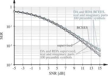
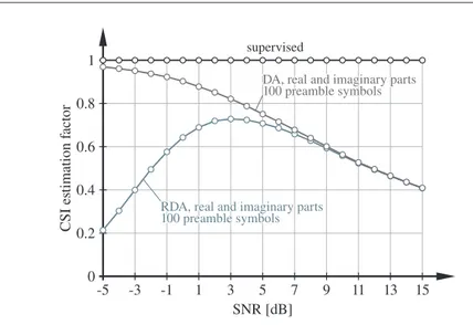
Considering preambles of 100 symbols, frames of 50 pilot symbols, and 250 user symbols, Figures 7 and 8 compare the results obtained with this refined decision rule, which is referred to asRefined Decision-Aided (RDA) criterion, considering an SNR threshold value oftSNR= 0 dB, to those obtained with the decision-aided approach. As it is shown in these figures, we can clearly conclude that applying the refined algorithm described in this section leads to a reduction in the CSI estimation factor for low SNR values and without penalizing the SER.

6 Conclusions

(10)

Acknowledgements This work has been funded by Xunta de Galicia, Ministerio de Ciencia e Innovaci´on of Spain, and FEDER funds of the European Union under grants with num-bers 10TIC105003PR, 10TIC003CT, 09TIC008105PR, TEC2010-19545-C04-01, and CSD2008-00010.

References

1. S. M. Alamouti. A Simple Transmit Diversity Technique for Wireless Communications.

IEEE Journal on Selected Areas in Communications, 16:1451–1458, 1998.

2. A. Bell and T. Sejnowski. An Information-Maximization Approach to Blind Separation and Blind Deconvolution. Neural Computation, 7(6):1129–1159, November 1995. 3. E. Beres and R. Adve. Blind Channel Estimation for Orthogonal STBC in MISO Systems.

InProc. of Global Telecommunications Conference (GLOBECOM 2004), volume 4, pages 2323–2328, 2004.

4. J. F. Cardoso and A. Souloumiac. Blind Beamforming for Non–Gaussian Signals. IEEE Proceedings-F, 140(6):362–370, 1993.

5. P. Comon and C. Jutten. Handbook of Blind Source Separation, Independent Component Analysis and Applications. Academic Press, 2010.

6. A. Dapena, H. P´erez-Iglesias, and V. Zarzoso. Blind Channel Estimation Based on Maxi-mizing the Eigenvalue Spread of Cumulant Matrices in (2 x 1) Alamouti’s Coding Schemes.

Wireless Communications and Mobile Computing, Article published online : 5 OCT 2010, DOI: 10.1002/wcm.992., 2010.

7. D. Gesbert, D. Shan-Shiu, P. J. Smith, and A. Nagui. From Theory to Practice: An Overview of MIMO Space-Time Coded Wireless Systems. IEEE Journal on Selected Areas in Communications, 21:281–302, 2003.

8. S. Haykin.Neural Networks A Comprehensive Foundation. Macmillan College Publishing Company, New York, 1994.

9. J. V. Stone.Independent Component Analysis: A Tutorial Introduction. MIT Press, 2004. 10. V. Tarokh, H. Jafarkhani, and A. R. Calderbank. Space-time Block Codes from Orthogonal

Designs.IEEE Transactions on Information Theory, 45(5):1456–1467, July 1999. 11. J. V´ıa, I. Santamar´ıa, J. P´erez, and D. Ram´ırez. Blind Decoding of MISO-OSTBC Systems

(11)

bi modulator S/P Alamouti coder s₁ s₂ s₁ s₂

-s₂*

s₁* z -1

x₁=z₁

x₂=z₂*

Alamouti decoder H

s=HH _x

s₁ s₂ ( )* z₁ z₂ h₁ h₂

Fig. 1 Alamouti coded scheme.

2500 2000 1500 1000 500 0 num be

r of oc

cur

re

nc

es

decision rule: real and imaginary parts (a) 10 preamble symbols

unchanged channel

threshold t = 0.2951 time-variant channel 1 0.9 0.8 0.7 0.6 0.5 0.4 0.3 0.2 0.1 0 2500 2000 1500 1000 500 0

difference in cross-correlation value

num

be

r of oc

cur

re

nc

es

(b) 100 preamble symbols (b) 100 preamble symbols

unchanged channel

threshold t = 0.1550

time-variant channel

(12)

2500

2000

1500

1000

500

0

num

be

r of oc

cur

re

nc

es

decision rule: absolute value squared (a) 10 preamble symbols

1 0.9 0.8 0.7 0.6 0.5 0.4 0.3 0.2 0.1 0 2500

2000

1500

1000

500

0

difference in cross-correlation value

num

be

r of oc

cur

re

nc

es

(b) 100 preamble symbols

(b) 100 preamble symbols unchanged channel

threshold t_{= 0.3650} time-variant channel

unchanged channel

threshold t_{= 0.1950}

time-variant channel

(13)

110 100 90 80 70 60 50 40 30 20 10 0.4

0.3

0.2

0.1

0

preamble size [number of symbols]

thr

es

hol

d

absolute value squared

real and imaginary parts

(14)

10-3 10-2 10-1 1

S

E

R

(a) supervised approaches

15 13 11 9 7 5 3 1 -1 -3 -5 10-3 10-2 10-1 1

SNR [dB]

S

E

R

(b) unsupervised approach

SNR [dB]

S

E

R

(b) unsupervised approach

DA-Supervised, absolute value squared 100 preamble symbols DA-Supervised,

absolute value squared 10 preamble symbols

supervised DA-Supervised, real and imaginary parts 100 preamble symbols

DA-Supervised, real and imaginary parts 10 preamble symbols

BCEES

DA-BCEES,

real and imaginary parts 100 preamble symbols

DA-BCEES,

(15)

15 13 11 9 7 5 3 1 -1 -3 -5 1 0.8 0.6 0.4 0.2 0 SNR [dB] CS I e st im at ion f ac tor supervised

real a_{nd i} magi

nary pa rts 10 pr

eam_{ble s} ym

bol s

absolute value squared 100 preamble symbols absolute value squared

10 preamble symbols

Fig. 6 Algorithm performance: CSI estimation factor versus SNR. The CSI estimation factor is evaluated as the ratio between the frames in which the channel is estimated and the total number of frames transmitted.

15 13 11 9 7 5 3 1 -1 -3 -5 10-3 10-2 10-1 1 SNR [dB] S E R

DA and RDA BCEES, real and imaginary parts 100 preamble symbols

supervised

BCEES

DA and RDA supervised, real and imaginary parts 100 preamble symbols

(16)

15 13 11 9 7 5 3 1 -1 -3 -5 1

0.8

0.6

0.4

0.2

0