A fully discrete BEM–FEM method for an
exterior elasticity system in the plane
Salim Meddahi
1and Mar´ıa Gonz´
alez
2Departamento de Matem´aticas, Universidad de Oviedo, Calvo Sotelo s/n, 33007–Oviedo, Spain
Abstract
We present a modified version of the usual BEM–FEM coupling for the exterior elasticity problem in the plane, cf. [7]. This new formulation allows us to take advantage of techniques from [13] to compute the boundary integral terms using simple quadrature formulas. We provide error estimates for the Galerkin method and prove that the corresponding fully discrete scheme preserves the optimal rates of convergence.
Key words: exterior boundary value problem; boundary element methods; finite element methods
1 Introduction
The idea of coupling the finite element method (FEM) and the boundary element method (BEM) consists in compensating the deficiencies of each method with the advantages of the other one. Indeed, the FEM can only be used on bounded domains while the BEM requires linear equations with constant coefficients. Often, it is necessary to combine both of them to solve problems in exterior domains.
Much progress has been made in the numerical analysis of these methods since the first BEM–FEM coupling was introduced at the beginning of the eighties, cf. [14]. However, a lot remains to be done before these coupling procedures become popular tools for engi-neering calculations. For example, little is known about efficient algorithms to solve the
1 The research of this author was supported by D.G.E.S. through the project PB98-1564. 2 The research of this author was supported by F.I.C.Y.T. through the project
complicated linear systems that arise from these formulations, cf. [16,10]. It is also diffi-cult to control the effect of numerical integration on the convergence of these methods. The main result of this paper concerns contributions to the analysis of a fully discrete BEM–FEM coupling for an exterior elasticity problem in the plane.
The most popular BEM–FEM formulations are the Johnson–Nedelec method (cf. [14]) and thesymmetric method (cf. [5,12]) which is used for the elasticity problem. It consists in dividing the exterior domain into a bounded inner region and an unbounded outer one by introducing an auxiliary common boundary. Next, the integral representation of the solution in the unbounded domain provides two non–local conditions on the auxiliary boundary for the problem in the inner region.
All authors (cf. [2],[9],[7]) choose a polygonal curve as an auxiliary boundary. At first glance, this election seems to be more suitable to deal with the discrete problem. How-ever, in this case, it is not known how to control the effect of numerical integration on convergence. In this paper, we use a regular curve as an artificial boundary (as in [16,17]) and substitute all terms on this boundary by the corresponding periodic functions. This modified BEM–FEM formulation of the elasticity problem is equivalent to the usual one at the continuous level but it leads to a different Galerkin method that admits a completely discrete version by using elementary quadrature formulas.
The rest of the paper is organized as follows. In section 2, we present a new version of the symmetric BEM–FEM formulation for the elasticity problem and show that the corresponding variational problem is well posed. In section 3, we describe the discretization of the problem and provide an error analysis for the Galerkin scheme. In section 4, we introduce a family of full discretizations of the complete system of equations. Finally, in section 5 we prove that these numerical integration schemes preserve the optimal rates of convergence.
Next we describe some notations used throughout this paper. LetO be an open set inR2. We use the Hilbertian Sobolev spacesHm(O) endowed with their usual normsk·k
m,O. The
inner product of L2(O) =H0(O) is denoted by (·,·)
0,O. Finally, the spaces Wm,∞(O) are
those Sobolev spaces derived fromL∞(O) (cf. [1]); we denote their norms and seminorms byk · km,∞,O and | · |m,∞,O, respectively.
We also consider periodic Sobolev spaces. Given a 1–periodicC∞ functiong, we define its
Fourier coefficients
ˆ g(k) :=
Z 1
0
g(s)e−2kπısds, ∀k ∈Z.
Then, for each real number r, the 1-periodic Sobolev space Hr is the completion of the
space of 1–periodic C∞ functions with respect to the norm
kgkr :=
|gˆ(0)|
2
+X
k6=0
|k|2r|gˆ(k)|2
1/2
It is well known (cf. [19] or [15]) that Hr is a Hilbert space for each r. Moreover, the
H0–inner product
(ξ, η) :=
Z 1
0
ξ(s)η(s)ds,
can be extended to represent the duality between H−r and Hr for each r. We will keep
the same notation for this duality bracket.
On the other hand, since we will deal with vector unknowns, we need product forms of some spaces. Let H be a normed space. Then, we denote by H := H ×H the product space endowed with the usual product norm and the corresponding inner product if it exists. We will use the same notation for the inner product and norm of the product space.
We denote vectors and vector–valued functions by small boldface letters. Matrices and matrix–valued functions are denoted by capital boldface letters. The superscript > will denote transposition of a matrix. Finally, we denote by a dot the Euclidean inner product inR2 and by a colon the Euclidean inner product inR2×2, the space of real 2×2 matrices, i.e.,
u·v:=
2
X
i=1
uivi, A:B:=
2
X
i,j=1
Ai,jBi,j.
In all what follows, C denotes a generic constant independent of the discretization pa-rameterh.
2 The model problem
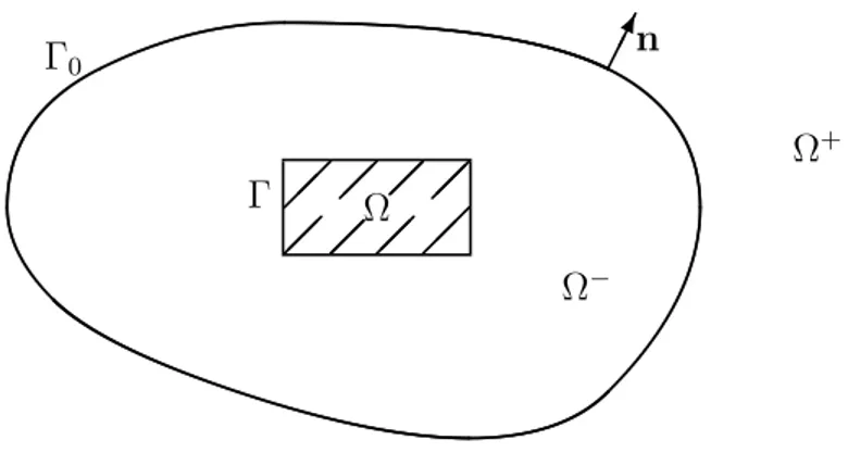
Let Ω be a bounded domain inR2 with Lipschitz boundary Γ and let us denote by Ω0 the
complement of its closure Ω in R2. Letf be a function with a compact support contained
in Ω0. We consider the exterior Dirichlet problem for the Lam´e system. This consists in finding a displacement vector u satisfying
−
2
X
j=1
∂Sij[u]
∂xj
=fi, in Ω0, i= 1,2,
u =0, on Γ,
u(x) = O(1), as |x| →+∞.
(1)
We denoted by S[u] the stress tensor
Ω
n
Ω−
Ω+ Γ
Γ0
Fig. 1. Geometry of the problem
whereλ≥0 and µ >0 are the Lam´e constants, Iis the identity matrix andE[u] denotes the strain tensor
Eij[u] :=
1 2
∂ui
∂xj
+ ∂uj ∂xi
!
, 1≤i, j ≤2.
Let Ω0be a simply connected bounded domain inR2 with a smooth boundary Γ0,
contain-ing both the support of f and Ω in its interior. The auxiliar boundary Γ0 divides Ω0 into
two subdomains, Ω− := Ω0∩Ω0 and Ω+ := Ω00. We denote the limit onto Γ0 of a function
defined on Ω+ or Ω− by the superscript + or −, respectively. Letn be the unit normal to
Γ0 oriented from Ω− to Ω+. We denote by t±[u] := S[u]±n the traction operator on Γ0.
Afterwards, problem (1) can be rewritten as an interior problem
−
2
X
j=1
∂Sij[u]
∂xj
= fi, in Ω−, i= 1,2,
u = 0, on Γ,
(2)
coupled with the exterior problem
−
2
X
j=1
∂Sij[u]
∂xj
= 0, in Ω+, i= 1,2,
u(x) = O(1), as |x| →+∞,
(3)
by means of the transmission conditions
u− = u+,
t−[u] = t+[u]. (4)
integrate over Ω− and apply a Green’s formula to obtain
a(u,v)−
Z
Γ0
t−[u]·vdσ= (f,v)0,Ω−, ∀v∈H1
Γ(Ω −
), (5)
whereH1Γ(Ω−) is the subspace of H1(Ω−) formed by those functionsv satisfying v|Γ =0
and
a(u,v) :=
Z
Ω−{λ(∇ ·u)(∇ ·v) + 2µE[u] :E[v]}dx, ∀u,v∈H
1
(Ω−).
The bounded bilinear forma(·,·) is elliptic onH1Γ(Ω−) by virtue of Korn’s inequality, i.e., there exists a constant α >0 such that
a(v,v)≥αkvk2
1,Ω−, ∀v∈H 1 Γ(Ω
−). (6)
LetU be the fundamental tensor of the Lam´e equation,
U(x,y) = − λ+ 3µ
4πµ(λ+ 2µ)log|x−y|I+
λ+µ 4πµ(λ+ 2µ)
(x−y)(x−y)>
|x−y|2 .
We denote by Ui the column vectors of Uand define
T±[U] := (t±[U1],t±[U2])>.
Then, we can represent the solution of problem (3) through the Betti–Somigliana formula:
u(x) =
Z
Γ0
T+y[U(x,y)]u+(y)dσy−
Z
Γ0
U(x,y)t+[u](y)dσy+c, ∀x∈Ω+, (7)
where c = (c1, c2)> is a constant. In relation (7) the subscript y in operator T+
de-notes differentiation with respect to the y variables and integration must be understood componentwise.
The symmetric method consists in coupling the variational formulation of the interior problem (5) with two boundary integral equations on Γ0. These boundary integral
equa-tions are derived from (7) and they relate the Cauchy data u and t[u] to each other on the artificial boundary Γ0.
Letting xapproach Γ0 in equation (7) and taking into account the jump relations of the
layer potentials (cf. [3]), we deduce the first boundary integral equation on Γ0:
1 2 u
+(x)−Z Γ0
T+y[U(x,y)]u+(y)dσy+
Z
Γ0
U(x,y)t+[u](y)dσy−c=0. (8)
The second equation is obtained by applying the traction operator to (7) and using the jump relations of the layer potentials (cf. [3]),
1 2t
+[u](x) =Z Γ0
(T+xhT+y[U(x,y)]i)>u+(y)dσy−
Z
Γ0
(T+x[U(x,y)])>t+[u](y)dσy. (9)
Here, the kernel of the first operator on the right hand side is hypersingular. The corre-sponding operator is obtained by a regularisation of the divergent integral by the usual procedure, cf. [3].
Letx: R−→R2 be a smooth regular 1-periodic parametric representation of Γ
0. We can
define the parameterized trace onto Γ0 as the unique extension of the mapping
γ : C∞(Ω−)−→ H0
u 7−→ γu(·) :=u◦x(·)
toH1(Ω−). By the trace theorem, γ: H1(Ω−)−→H1/2 is bounded and onto, cf. theorem 8.15 in [15].
The parameterized versions of the simple and double layer potentials are given by:
(Vη)(s) :=
Z 1
0
V(s, t)η(t)dt, (Kη)(s) :=
Z 1
0
K(s, t)η(t)dt,
where V(s, t) :=U(x(s),x(t)) and
K(s, t) = |x0(t)|T+x(t)[U(x(s),x(t))]
= µ|x
0(t)|
2π(λ+ 2µ)
(x(s)−x(t))·n(x(t))
|x(s)−x(t)|2 I−
(x(s)−x(t))·τ(x(t))
|x(s)−x(t)|2 eI
!
+ λ+µ π(λ+ 2µ)|x
0
(t)|(x(s)−x(t))(x(s)−x(t))
>
|x(s)−x(t)|4 (x(s)−x(t))·n(x(t)).
Here, τ is the tangent vector to Γ0 and eI=
0 −1 1 0
.
In the sequel, we denote
ξ(t) :=|x0(t)|t+[u](x(t)).
Using the representation formula (7), one can easily show that the behaviour of u at infinity is equivalent to a zero mean–value condition on t+[u](x) on Γ
0. It follows that
Z 1
0
ξ(s)ds=
Z
Γ0
Then, parameterising equation (8), we obtain the following periodic integral equation:
(1
2I − K)γu
++Vξ−c=0, (10)
where I denotes the identity operator andγ is applied componentwise.
On the other hand, we recall the following relation from Gwinner and Stephan (cf. [11])
Z
Γ0
(T+xhT+y[U(x,y)]i)>u+(y)dσy = ∂ ∂τ(x)(
Z
Γ0
U∗(x,y)∂u
+(y)
∂τ(y) dσy),
where
U∗(x,y) = µ(λ+µ)
π(λ+ 2µ) {−log|x−y|I+
(x−y)(x−y)>
|x−y|2 }.
Making use of the parameterization x(·), we obtain
−
Z
Γ0
(
Z
Γ0
(T+xhT+y[U(x,y)]i)>u+(y)dσy)v(x)dσx = ( d dsγv,V
∗ d
dsγu
+
), (11)
for all v∈ C∞(Ω−)2, where operator V∗ is formally given by
(V∗ξ)(s) :=
Z 1
0
V∗(s, t)ξ(t)dt, with V∗(s, t) := U∗(x(s),x(t)).
Then, combining equations (9) and (5) and using relation (11), we obtain
a(u,v) + ( d dsγv,V
∗ d
dsγu
+)−((1
2I − K
0
)ξ, γv) = (f,v)0,Ω−, ∀v∈H1
Γ(Ω −
), (12)
where K0 is the adjoint ofK.
Let H0−1/2 be the subspace of H−1/2 formed by those functions η satisfying (η,1) = 0.
Putting together equations (12) and (10) and using the transmission conditions (4) we obtain a weak formulation of problem (1):
find (u,ξ)∈H1 Γ(Ω
−)×H−1/2
0 such that
a(u,v) +b∗(d dsγu,
d
dsγv)−c(v,ξ) = (f,v)0,Ω−, ∀v∈H
1 Γ(Ω
−),
c(u,η) +b(ξ,η) = 0, ∀η∈H−10 /2,
(13)
where we denoted
b(ξ,η) = (η,Vξ), b∗(ξ,η) = (η,V∗ξ) and c(v,η) = (η,(1
To prove that problem (13) is well posed we need the following properties of the integral operators V, K and V∗ defined before.
Lemma 1 Operators V: H−1/2 → H1/2, K: H1/2 → H1/2 and V∗: H−1/2 → H1/2 are
linear and bounded. Furthermore, there exists a constant β >0 such that
(η,Vη)≥βkηk2
−1/2, ∀η∈H −1/2
0 (14)
and the operator −d dsV
∗ d ds: H
1/2 −→H−1/2 is nonnegative, i.e.,
(dg ds,V
∗ dg
ds)≥0, ∀g∈H
1/2. (15)
PROOF. One can easily show that both V and K inherit the properties of the clas-sical simple and double layer potentials proved in [7] or [3]. On the other hand, as γ: H1(Ω−) −→ H1/2 is onto, for any g ∈ H1/2, there exists a function u ∈ H1(Ω−)
such that γu=g and by virtue of relation (11),
(dg ds,V
∗ dg
ds) = −
Z
Γ0
(
Z
Γ0
(T+x[T+y[U(x,y)]])>u(y)dσy)u(x)dσx
where the right hand side is nonnegative (cf. [7]).
We denote by M the product space H1Γ(Ω−)×H−10 /2 endowed with its natural inner product and the induced normk·kM. Consider the bounded bilinear formA: M×M−→R obtained by adding the left hand sides of (13), i.e.,
A(ˆu,v) =ˆ a(u,v) +b∗( d dsγu,
d
dsγv)−c(v,ξ) +b(ξ,η) +c(u,η),
where we denoted the elements of M by ˆu := (u,ξ) and ˆv := (v,η). It turns out that A(·,·) is M–elliptic since (6), (14) and (15) give
A(ˆv,v)ˆ ≥αkvk2
1,Ω−+βkηk−12 /2 ≥α˜kvˆk2M, ∀vˆ= (v,η)∈M, (16) with ˜α:= min{α, β}. Let L: M−→R be the bounded linear functional defined by
L(ˆv) = (f,v)0,Ω−, ∀vˆ = (v,η)∈M.
With these notations, problem (13) may be written
find ˆu∈M such that
A(ˆu,v) =ˆ L(ˆv), ∀vˆ ∈M.
(17)
3 The discrete problem
3.1 Curved triangulation of the bounded domain
For simplicity of exposition we assume that Γ is a polygonal curve. Given a positive integer N andh:= 1/N, let{si :=i h; i= 0,· · · , N}be the induced uniform partition of [0,1].
We denote by Ωh the polygonal domain whose vertices lying on Γ0 are ∆h :={x(si)}Ni=1.
Let τh be a triangulation of Ωh by triangles T of diameter hT not greater than Ch. We
assume that any vertex of a triangle lying on the exterior boundary of Ωh belongs to ∆h.
We also suppose that the family of triangulations {τh}h is regular in the sense of [4].
We obtain from τh a triangulationτh− of Ω
−
by replacing each triangle of τh with one side
along the exterior part of ∂Ωh by the corresponding curved triangle.
LetT be a curved triangle ofτh−. We denote its vertices byP1,T,P2,T andP3,T, numbered
in such a way that there exists an index i such that x(si−1) = P2,T and x(si) = P3,T.
Then, the mapping ϕ : [0,1]→R2 defined by
ϕ(s) :=x(si−1+s h), s ∈[0,1],
is a parameterization of the curved side of T.
LetTb be the reference triangle with verticesPb1 := (0,0)>,Pb2 := (1,0)>andPb3 := (0,1)>.
Consider the affine mapping GT defined by GT(Pbi) = Pi,T for i ∈ {1,2,3} and the
function ΘT :Tb →R2 given by
ΘT(ˆx) :=
ˆ x1
1−xˆ2
(ϕ(ˆx2)−(1−xˆ2)P2,T −xˆ2P3,T), ∀xˆ = (ˆx1,xˆ2)∈T ,b
where the limiting value has to be taken when ˆx2 tends to 1. We then introduce the C∞
mapping FT :Tb →R2 given by
FT :=GT +ΘT.
It is proved in theorem 22.4 of [20] that FT is a C∞–diffeomorphism from Tb onto T.
Moreover, ΘT(0, s) = ΘT(s,0) = (0,0)> and FT(s,1−s) = ϕ(s) for all s ∈ [0,1]. Then
each side of Tb is mapped onto the corresponding side of T.
On each curved triangleT, a finite element may be defined by the triplet (T, P1(T),ΣT),
where P1(T) is the space of functions defined on T with pullback in the space P1 of
polynomials of degree not greater than one:
P1(T) :={p:T →R : p◦FT ∈P1}
and ΣT :={Ni,T : i= 1,2,3} is the set of Lagrange functionals: Ni,T(φ) :=φ(Pi,T). It is
side of T, a functionφ ∈P1(T) is uniquely determined by its nodal values corresponding
to that side. On straight triangles we use the classical P1-finite element.
Under the assumption of regularity of {τh}, theorem 22.4 in [20] proves that, for curved
triangles T, the Jacobian JT of FT does not vanish on a neighborhood of Tb and the
following estimates hold:
C1h2T ≤ |JT(·)| ≤C2h2T, (18)
|FT|k,∞, b T ≤Ch
k
T, k = 1,2, (19)
|F−1T |1,∞,T ≤Ch−1T . (20)
These properties of FT and the usual technique used in the affine case permit to obtain
interpolation error bounds on curved triangles (cf. section 4.3 of [4]). Namely, there exists a constantC independent of T such that
|v −πTv|1,T ≤ ChTkvk2,T ∀v ∈H2(T), (21)
whereπTv ∈P1(T) and is uniquely determined byπTv(Pi,T) = v(Pi,T) for i= 1,2,3.
No-tice that in the case of straight triangles, we obtain the same estimate with the seminorm of H2(T) instead of the norm on the right hand side.
3.2 Discrete spaces and Galerkin scheme
We will seek the approximate displacement field in
Vh :={vh ∈ C0(Ω
−
,R2) :vh|T ∈P1(T), ∀T ∈τh−} ∩H
1 Γ(Ω
−
),
where, as usual, P1(T) = P1(T)×P1(T). On the other hand, we define
Hh :={ηh ∈L
2(0,1) : η
h|(si−1,si)∈P0, i= 1, . . . , N} ∩H
−1/2
0 ,
where P0 is the space of constant functions.
The discrete problem associated to the variational formulation (13) consists in finding (uh,ξh)∈Vh×Hh such that
a(uh,vh) +b∗(
d
dsγ(uh), d
dsγ(vh))−c(vh,ξh) = (f,vh)0,Ω−, ∀vh ∈Vh,
c(uh,ηh) +b(ξh,ηh) = 0, ∀ηh ∈Hh.
Let us introduce the space Mh :=Vh×Hh. Problem (22) can be equivalently written
find ˆuh ∈Mh such that
A(ˆuh,vˆh) =L(ˆvh), ∀vˆh ∈Mh.
(23)
The ellipticity of A(·,·) implies that this problem is well posed and we have the following C´ea’s inequality:
ku−uhk1,Ω−+kξ−ξhk−1/2 ≤C( inf vh∈Vh
ku−vhk1,Ω−+ inf ηh∈Hh
kξ−ηhk−1/2). (24)
Theorem 2 If u belongs to H2(Ω−) then
ku−uhk1,Ω−+kξ−ξ
hk−1/2 ≤Chkuk2,Ω−.
PROOF. The local interpolation error estimates (21) lead to the following inequality:
inf vh∈Vh
kv−vhk1,Ω− ≤Chkvk2,Ω−, ∀v∈H1Γ(Ω−)∩H2(Ω−) (25)
and classical approximation properties in periodic Sobolev spaces (cf. [18]) give
inf
ηh∈Hh
kη−ηhk−1/2 ≤Chkηk1/2, ∀η∈H −1/2
0 ∩H1/2. (26)
We deduce the result from inequalities (25) and (26) together with (24) and the trace theorem.
4 Full discretization of the equations
In this section, we describe the different quadratures used to approximate the integrals in (22). We begin by the interior terms. Let Qb be a quadrature formula on the reference
triangleTb:
b
Q(ϕ) :=
d0
X
k=1
ˆ
ωkϕ(ˆbk)' Z
b T
ϕ(ˆx)dxˆ.
We assume thatQb is exact for constant functions; i.e.,Pd0
k=1ωˆk = 1/2. The corresponding
formulaQT on a given triangle T ∈τh− is obtained by a simple change of variable
QT(φ) := Qb(|JT|φˆ) = d0
X
k=1
ˆ
ωk|JT|(ˆbk) ˆφ(ˆbk)' Z
T
where we denoted ˆφ:=φ◦FT. We approximate the linear form L(·) by
Lh(ˆvh) := X
T∈τh−
QT(f ·vh)
onMh and the bilinear form a(·,·) by
ah(uh,vh) := X
T∈τh−
QT(λ(∇ ·uh)(∇ ·vh) + 2µE[uh] :E[vh])
onVh×Vh.
For the boundary terms, we need a basic quadrature formula on the unit square:
ˆ `2(g) :=
d1
X
k=1
ηkg(xk)' Z 1
0
Z 1
0
g(s, t)dsdt.
We assume that ˆ`2 is exact for polynomial functions of degree not greater than one. In
the following, we introduce three different types of approximations:
1. Numerical quadratures must be handled with care when defining an approximation ofb(·,·) onHh×Hh because of the logarithmic singularity ofV. Here, we follow [13] and
consider the following decomposition of the kernel:
V(s, t) = −Cλ,µ log|s−t|2 I+B(s, t),
where Cλ,µ = 8πµλ(+3λ+2µµ). Notice that the matrix valued function B(·,·) is of class C∞ in
the domain D1 ={(s, t)∈[0,1]×[0,1] :|s−t| <1}. Now, the strategy consists in using
ˆ
`2 to approximate the second integral and compute the first one exactly (cf. [13] or [8]);
i.e.,
Z si
si−1
Z sj
sj−1
V(s, t)ds dt'Vi,j :=h2
ˆ
`2(B(si−1+h·, sj−1+h·))−Cλ,µ(logh2+Bi−j)I
,
with
Bk:= Z 1
0
Z 1
0
log|k+t−s|2dt ds, ∀k ∈Z
and
(i, j) :=
(i, j), if |i−j| ≤ N/2, (i, j+N), if i−j > N/2, (i, j−N), if j−i > N/2.
Let us denoteηithe constant value of a given functionη
h ∈Hh on (si−1, si), (1≤i≤N).
Then, for any ξh, ηh ∈Hh, we define
bh(ξh,ηh) := N X
i,j=1
(ηi)>Vi,jξj.
2. Notice that if uh is a function inVh, then γuh belongs to the space Th, where
Th ={ηh ∈ C0(R) : ηh|(si−1,si) ∈P1, 1≤i≤N; ηh(s) = ηh(s+ 1), ∀s ∈R}.
Hence, for any vh ∈Vh, dsdγvh ∈ Hh and it suffices to approximate b∗(·,·) on Hh×Hh
by the same technique given in the previous case. Indeed, the singularity of V∗(·,·) is removed as above to obtain
Z si
si−1
Z sj
sj−1
V∗(s, t)'V∗i,j :=h2`ˆ2(B∗(si−1+h·, sj−1+h·))−Cλ,µ∗ (logh2+Bi−j)I
,
where Cλ,µ∗ = 2µπ((λλ++2µµ)) and B∗(·,·) is a matrix–valued function of class C∞ in the domain
D1. Afterwards, we define the perturbed bilinear form
b∗h(ξh,ηh) :=
N X
i,j=1
(ηi)>V∗i,jξj.
3. It remains to define an approximation ch(vh,ηh) ofc(vh,ηh) onVh×Hh. Let{`i}Ni=1
be the set of nodal basis functions of Th, i.e., `i(sj) = δi,j, for all 1 ≤i, j ≤N. Thus, it
suffices to provide a quadrature scheme for
Z si
si−1
Z sj+1
sj−1
`j(t)K(s, t)dt ds, (27)
where sN+1 = 1 +h.
To treat the singularity of the kernel of operator Kwe use the decomposition
K(s, t) = − µ
2π(λ+ 2µ) 1
s−t eI+C(s, t).
Notice that C(·,·) is a matrix–valued function of class C∞. Then (27) writes
− µ
2π(λ+ 2µ)
Z si
si−1
Z sj+1
sj−1
1
s−t `j(t)eIdt ds+
Z si
si−1
Z sj+1
sj−1
Computing the first term of (28) exactly we obtain
Z si
si−1
Z sj+1
sj−1
1
s−t `j(t)eIdt ds= h
2 Ai−jeI,
where the coefficients Ak are determined by the conditions:A−k =−Ak+1 ∀k ∈N, and
Ak = (k+1)2log(1−
1
k2)−4(k+
1
2) log(1− 1 k)−k
2log(1− 1
(k−1)2)+4(k−1) log(1−
1 k−1),
for k > 2 with A1 = 4 log 2 and A2 = 9 log 3− 12 log 2. The second term of (28) is
approximated by h2`ˆ2(Ci j), where we denoted
Ci j(s, t) := `j(sj−1 +ht)C(si−1+hs, sj−1+ht) +`j(sj+ht)C(si−1+hs, sj +ht).
It follows that
ch(vh,ηh) =
1
2(ηh, γvh)−
N X
i,j=1
(ηi)>h2`ˆ2(Ci j)−
µ 2π(λ+ 2µ)
h
2 Ai−jeI
γvh(sj).
We are now in a position to write the fully discrete scheme associated to problem (13),
find u∗h ∈Vh and ξ∗h ∈Hh;
ah(u∗h,vh) +b∗h(
d dsγu
∗
h,
d
dsγvh)−ch(vh,ξ
∗
h) = Lh(vh), ∀vh ∈Vh,
bh(ξ∗h,ηh) +ch(u∗h,ηh) = 0, ∀ηh ∈Hh.
(29)
5 Analysis of the fully discrete scheme
In this section, we study the stability and convergence of the fully discrete scheme (29). We begin with some bounds related to the five kinds of approximations presented in the last section.
The following results concern estimates on the error committed when approximating the right hand side and the energy form a(·,·). They follow readily from lemma 26.7 and lemma 26.6 in [20].
Lemma 3 If f ∈W1,∞(Ω−), then there exists a constant C independent of h such that
Lemma 4 There exists a constant C independent of h such that
|a(uh,vh)−ah(uh,vh)| ≤Chkuhk1,Ω−kvhk1,Ω−, ∀uh,vh ∈Vh.
For the bilinear forms associated to the boundary integral operators we have the following results.
Lemma 5 There exists a constant C independent of h such that
|b(ξh,ηh)−bh(ξh,ηh)| ≤Chkξhk−1/2kηhk−1/2, ∀ξh,ηh ∈Hh.
PROOF. See lemma 11 in [8].
Lemma 6 There exists a constant C independent of h such that
|b∗( d dsγuh,
d
dsγvh)−b
∗
h(
d dsγuh,
d
dsγvh)| ≤Chkuhk1,Ω−kvhk1,Ω−, ∀uh,vh ∈Vh.
PROOF. Lemma 5 shows that there exists a constantC > 0 such that
|b∗(ξh,ηh)−b∗h(ξh,ηh)| ≤Chkξhk−1/2kηhk−1/2, ∀ξh,ηh ∈Hh.
Therefore,
|b∗( d dsγuh,
d
dsγvh)−b
∗
h(
d dsγuh,
d
dsγvh)| ≤Chk d
dsγuhk−1/2k d
dsγvhk−1/2
and the boundness of operators d ds:H
1/2 −→H−1/2 and γ imply the result.
Lemma 7 There exists a constant C independent of h such that
|c(vh,ηh)−ch(vh,ηh)| ≤Ch
3/2kv
hk1,Ω−kηhk−1/2, ∀vh ∈Vh, ∀ηh ∈Hh.
PROOF. For anyvh ∈Vh and ηh ∈Hh we have
c(vh,ηh)−ch(vh,ηh) =h2 N X
i,j=1
(ηi)>eˆ2(Ci j)γvh(sj),
where ˆe2(·) :=
R1 0
R1
0 · −`ˆ2(·) is the error functional. Since ˆ`2 is of degree 1 on D :=
(0,1)×(0,1), it follows readily from the Bramble-Hilbert lemma that
and the chain rule shows that
|Ci j|2,∞,D ≤Ch2kCk2,∞,D,
Therefore, we have the following estimate
|c(vh,ηh)−ch(vh,ηh)| ≤Ch
4kCk 2,∞,D
N X
i=1
|ηi|
N X
j=1
|γvh(sj)|.
On the other hand, a well known inverse inequality leads to
h
N X
i=1
|ηi|=
Z 1
0
|ηh(s)|ds≤ kηhk0 ≤Ch−1/2kηhk−1/2 ∀ηh ∈Hh
and the equivalence of the norms g → kgk0 and g → (hPNi=1g(ti)2)1/2 on Th together
with the trace theorem provide
N X
j=1
|γvh(sj)| ≤h−1
h N X
j=1
|γvh(sj)|2
1/2
≤Ch−1kγvhk0 ≤Ch−1kvhk1,Ω−.
The result is now a direct consequence of the last inequalities.
We introduce the bilinear form
Ah(ˆuh,vˆh) = ah(uh,vh) +b∗h(
d dsγuh,
d
dsγvh)−ch(vh,ξh) +bh(ξh,ηh) +ch(uh,ηh), for all ˆuh = (uh,ξh) and ˆvh = (vh,ηh) inMh. Using the triangular inequality and lemmas
4–7 we deduce the following estimate.
Corollary 8 There exists a positive constant C such that
|A(ˆuh,vˆh)−Ah(ˆuh,vˆh)| ≤ChkuˆhkMkvˆhkM, ∀uˆh,vˆh ∈Mh.
This allows us to prove that, if h is sufficiently small,Ah(·,·) is uniformly elliptic on Mh
since
Ah(ˆvh,vˆh)≥(αe−Ch)kvˆhk
2
M, ∀vˆh ∈Mh.
Thus, problem (29), which may be equivalently written
find ˆu∗h ∈Mh such that
Ah(ˆu∗h,vˆh) =Lh(ˆvh), ∀vˆh ∈Mh,
Theorem 9 If f ∈W1,∞(Ω−) and u∈H2(Ω−), then there exists a constant C > 0 such
that
ku−u∗hk1,Ω−+kξ−ξ∗
hk−1/2 ≤Ch(kuk2,Ω−+kfk1,∞,Ω−).
PROOF. As a consequence of Strang’s lemma (cf. [4]) we have the error estimate
kuˆ−uˆ∗hkM ≤C kuˆ−vˆhkM+ sup
ˆ
zh
|A(ˆvh,ˆzh)−Ah(ˆvh,zˆh)|
kˆzhkM
+ sup
ˆ
zh
|L(ˆzh)−Lh(ˆzh)|
kˆzhkM
!
,
for all ˆvh ∈Mh. Hence, the result follows from lemma 3, corollary 8 and the approximation
properties (25) and (26).
References
[1] R. Adams,Sobolev spaces (Academic Press, 1975).
[2] C. Carstensen, S.A. Funken and E.P. Stephan, On the adaptive coupling of FEM and BEM in 2-d-elasticity,Numer. Math. 77 (1997) 187–221.
[3] C. Chen and J. Zhou, Boundary element methods (Academic Press, London, 1992).
[4] Ph. G. Ciarlet, The Finite Element Method for Elliptic Problems (North-Holland, Amsterdam, 1978).
[5] M. Costabel, Symmetric methods for the coupling of finite elements and boundary elements, The Mathematics of Finite Elements and Applications IV (Academic Press, London, 1988).
[6] M. Costabel, Boundary integral operators on Lipschitz domains: Elementary results, SIAM J. Math. Anal.19 (1988) 613–626.
[7] M. Costabel and E.P. Stephan, Coupling of finite and boundary element methods for an elastoplastic interface problem,SIAM J. Numer. Anal. 27 (1990) 1212–1226.
[8] M. Crouzeix and F.-J. Sayas, Asymptotic expansions of the error of spline Galerkin boundary element methods.Numer. Math. 78(1998) 523–547.
[9] G.N. Gatica and G.C. Hsiao, Boundary–field equation methods for a class of nonlinear problems (Pitman Research Notes in Math.,331, Longman, 1995).
[10] G.N. Gatica and S. Meddahi, An a–posteriori error estimate for the coupling of BEM and mixed FEM,Technical Report 98–16, Departamento de Ingenier´ıa Matem´atica Universidad de Concepci´on, Chile (to appear in Numerical Functional Analysis and Optimization).
[12] H. Han, A new class of variational formulations for the coupling of finite and boundary element methods,J. Comput. Math. 8 (1990) 223–232.
[13] G.C. Hsiao, P. Kopp and W.L. Wendland, A Galerkin collocation method for some integral equations of the first kind,Computing 25(1980) 557–566.
[14] C. Johnson and J.C. N´ed´elec, On the coupling of boundary integral and finite element methods,Math. of Comp. 35 (1980) 1063–1079.
[15] R. Kress,Linear integral equations (Springer-Verlag, New York-Berlin, 1989).
[16] S. Meddahi, An optimal iterative process for the Johnson-N´ed´elec method of coupling boundary and finite elements. SIAM J. Numer. Anal. 35(1998) 1393–1415.
[17] S. Meddahi and F.-J. Sayas, A fully discrete BEM–FEM for the exterior Stokes problem in the plane,Publicaciones del Seminario Matem´atico Garc´ıa de Galdeano To appear in SIAM J. Numer. Anal.
[18] I.H. Sloan, Error analysis of boundary integral methods, in: A. Iserles ed., Acta Numerica (University Press, Cambridge, 1992) 287–339.
[19] Y. Yan, I.H. Sloan, On integral equations of the first kind with logarithmic kernels, J. Int. Eqns. Appl. 1(1988) 549–579.