TítuloA minimum weight with stress constraints FEM approach for topology structural optimization problems

(1)

"A minimum weight with stress constraints FEM approach for topology structural optimization problems"

I Muiños, I. Colominas, F. Navarrina, M. Casteleiro (2002)

(2)

WCCM V Fifth World Congress on Computational Mechanics July 7–12, 2002, Vienna, Austria Eds.: H.A. Mang, F.G. Rammerstorfer, J. Eberhardsteiner

A Minimum Weight with Stress Constraints FEM Approach

for Topology Structural Optimization Problems

Iago Mui ˜nos, Ignasi Colominas, Ferm´ın Navarrina, Manuel Casteleiro∗

GMNI — Grupo de Métodos Numéricos en Ingenier´ıa, Department of Applied Mathematics, Universidad de A Coruña,

E.T.S. de Ingenieros de Caminos, Canales y Puertos Campus de Elvi˜na, 15192 A Coru˜na, SPAIN

e-mail: [email protected], web page: http://caminos.udc.es/gmni

Key words: Topology Optimization, Design Optimization, Optimum Design, Structural Optimum

De-sign, Structural Optimization

Abstract

Sizing and shape structural optimization problems are normally stated in terms of a minimum weight approach with constraints that limit the maximum allowable stresses and displacements.

However, topology structural optimization problems have been traditionally stated in terms of a maxi-mum stiffness (minimaxi-mum compliance) approach. In this kind of formulations, the aim is to distribute a given amount of material in a certain domain, so that the stiffness of the resulting structure is maximized (the compliance, or energy of deformation, is minimized) for a given load case. Thus, the material mass is restricted to a predefined percentage of the maximum possible mass, while no stress or displacement constraints are taken into account.

(3)

1 Introduction

Around four decades ago Schmidt [1] proposed a revolutionary idea that gave rise to a new discipline: engineers, as a general rule, try to design minimum cost objects or systems that must withstand the max-imum unfavorable estimated loads; therefore, (optmax-imum) design could be systematically stated in terms of constrained minimization problems; then, these problems could be solved by means of mathematical programming techniques implemented in high speed digital computers. Sizing and shape structural opti-mization problems have been thereafter mainly written in terms of minimum weight formulations, with non linear constraints that limit the maximum allowable stresses and displacements [2, 3, 4].

However, since Bendsøe and Kikuchi proposed the basic concepts [5] in 1988, most of topology structural optimization problems have been routinely stated in terms of minimum compliance (maximum stiffness) approaches. In this kind of formulations, one tries to distribute a given amount of material within a given domain, so that the stiffness of the resulting structure is maximized (the compliance is minimized) for a given load case [6]. The traditional minimum compliance formulations offer some obvious advantages, since one avoids dealing with a large number of highly non-linear constraints. This could be considered crucial, if one takes into account the large number of design variables that is inherent to topology opti-mization. However, one can also argue that this gives rise to several important drawbacks. Thus, multiple load cases can not be considered, different solutions are obtained for different restrictions on the amount of material, and the final design could be unfeasible in practice, since no constraints are imposed on stresses and displacements. Moreover, the minimum compliance problem is said to be ill-posed, since the solution oscillates as the discretization refinement is increased [7, 8], although this difficulty can be partially overcome by introducing porous materials.

The SIMP (solid isotropic material with penalty) formulation [7, 8, 9] is the most widely used minimum compliance approach, so far. In this formulation, one introduces a non-dimensional design variable per element (the relative density, that is the one’s complement of the porosity), which value ranges from0

to1. The aim is to compute the design variables (the amount of porous material that must be distributed within each element) in such a way that a highly non-linear objective function is minimized (the compli-ance, or energy of deformation), while a single linear constraint is satisfied (the total amount of material is limited, by the so called filling factor, to occupy a predefined percentage of the domain volume). The SIMP formulation is easy to implement in a FEM framework. Moreover, several explicit procedures have been proposed to iterate the relative density of the elements [7, 8], what facilitates solving the minimiza-tion problem. However, a spread porous material distribuminimiza-tion is frequently considered an unwanted result, and numerical instabilities do often occur. Therefore, additional penalization and stabilization techniques must still be employed [7, 8]. On the other hand, an image filter is generally applied, in order to enable the final interpretation of the results. These normally resemble truss-like structures [7].

But one could question these results, since the final design depends on so many arbitrary parameters (filling factor, degree of discretization, applied penalization and stabilization techniques, image filter, etc.) One could even say that the final results are somehow impelled to resemble truss-like structures, since this is what one expects to obtain as a satisfactory final design. On the other hand, the final design could be unfeasible in practice, since the formulation disregards the stress and displacement fields. And, obviously, the stiffest design that can be built with a given amount of material will normally differ from the cheapest (in cost of material) design that can support a set of given load cases.

(4)

WCCM V, July 7–12, 2002, Vienna, Austria

2 The Structural Analysis Model

2.1 The Structural Analysis Problem

LetΩobe a domain in the material space originally occupied by a certain deforming body. Due to given external loads the body is deformed onto a different domainΩ. Thus, every arbitrary pointPo inΩois carried into a different positionPinΩ. Letrrrrrrrrrrrrrroandrrrrrrrrrrrrrrbe the material coordinates vectors of pointsPoand P, respectively. Our aim is to compute the displacements

u u uuuuu u

uuuuuu(rrrrrrrrrrrrrro) =rrrrrrrrrrrrrr(rrrrrrrrrrrrrro)−rrrrrrrrrrrrrro, (1) which are the key to obtain the deformationsεεεεεεεεεεεεεε(rrrrrrrrrrrrrro)and the stressesσσσσσσσσσσσσσσ(rrrrrrrrrrrrrro). In linear elasticity with small displacements and small deformations the corresponding expressions are

ε ε ε ε εεε ε ε ε εε ε

ε=LLLLuLLLLLLLLLLuu,uuuuuuuuuuu σσσσσσσσσσσσσσ=DDDεDDDDDDDDDDDεε.εεεεεεεεεεε (2)

Let the external loads be the forcesbbbbbbbbbbbbbb(rrrrrrrrrrrrrro)per unit volume (of the body) in the domainΩo, andtttttttttttttt(rrrrrrrrrrrrrro)per unit area on the surfaceΓo_σ. In these terms, the structural analysis problem can be written as [12, 13]

Find uuuuuuuuuuuuuu∈ Hu such that a(wwww, uwwwwwwwwww uuuuuuuuuuuuu) = (wwwwwwwwwwwww, bbbbbbbw bbbbbbb)Ωo + (wwwww, ttttttttttttttwwwwwwwww )_Γo

σ ∀wwwwwwwwwwwwww∈ Hw

being a(ww, uwwwwwwwwwwww uuuuuuuuuuuuu) =

ZZZ

Ωo

(LLwLLLLLLLLLLLLwwwwwwwwwwwww)TDDDDDDDDDDDDDD(LLuLLLLLLLLLLLLuuuuuuuuuuuuu)dΩ,

(ww, bbbbbbbwwwwwwwwwwww bbbbbbb)Ωo = ZZZ

Ωo

w w wwwww w

wwwwwwTbbbbbbb dbbbbbbb Ω, (ww, ttttttttttttttwwwwwwwwwwww )Γo

σ = ZZ Γo σ w w w w www w w w ww w wTtttttttttttttt dΓ,

(3)

where the trial functionsuuuuuuuuuuuuuuand the test functionswwwwwwwwwwwwwware required to satisfy the essential boundary condi-tions (prescribed displacements) and their corresponding homogeneus boundary condicondi-tions, respectively.

2.2 The Finite Element Numerical Model

As a general rule, it will not be possible to obtain the exact solution of the above stated problem. Hence, we will try to approximate the exact solution in a finite-dimensional context. Thus, we replace the func-tion spacesH_u andH_w by their respective finite dimension subspacesHh

u andHhw. Letuuuuuuuuuuuuuuh andwwwwwwwwwwwwwwh be

the discretized trial and test functions in the above mentioned subespaces. Let uuuuuuuuuuuuuup be a trial function that satisfies the essential boundary conditions. And let{φi(rrrrrrrrrrrrrro)}and{wj(rrrrrrrrrrrrrro)}be conveniently selected

bases of discretized trial and test functions in the corresponding subespacesHh

u andHwh, verifying the

homogeneus boundary conditions of our problem. In this terms we can write [12, 13]

u u u u uuu u u u uu u

uh(rrrrrrrrrrrrrro) =uuuuuuuuuuuuuup(rrrrrrrrrrrrrro) +

N X i=1 Φ Φ Φ Φ ΦΦΦ Φ Φ Φ ΦΦ Φ

Φi(rrrrrrrrrrrrrro)ααααααααααααααi, ΦΦΦΦΦΦΦΦΦΦΦΦΦΦi(rrrrrrrrrrrrrro) =φi(rrrrrrrrrrrrrro)IIIIIIIIIIIIII3,

w w w w www w w w ww w

wh(rrrrrrrrrrrrrro) =

N X j=1 W W W W W WW W W W W W W

Wj(rrrrrrrrrrrrrro)ββββββββββββββj, WWWWWWWWWWWWWWj(rrrrrrrrrrrrrro) =wj(rrrrrrrrrrrrrro)IIIIIIIIIIIIII3.

(4)

In a FEM formulation the unknownααααααααααααααi is the nodal displacements vector of node numberi. Moreover,

the domainΩois discretized in such a way that

¯ Ωo =

nelem

[

e=1

¯

Ee, Ee1 \

Ee2 =∅ ∀e16=e2, (5)

(5)

beingEe the so-called finite elements. On the other hand, in solid mechanics one normally resorts to a

Galerkin type formulation, by taking the same base for both, the trial and the test functions. Thus,

wj(rrrrrrrrrrrrrro) =φj(rrrrrrrrrrrrrro). (6)

Therefore, the FEM numerical model of structural analysis can be written as

Find αααααααααααααα={ααααααααααααααi}, i= 1, . . . , N such that N

X

i=1

K K KKKKK K

KKKKKKjiααααααααααααααi =ffffffffffffffj, j= 1, . . . , N

being KKKKKKKKKKKKKKji =a(ΦΦΦΦΦΦΦΦΦΦΦΦΦΦj,ΦΦΦΦΦΦΦΦΦΦΦΦΦΦi), ffffffffffffffj = (ΦΦΦΦΦΦΦΦΦΦΦΦΦΦj, bbbbbbbbbbbbbb)Ωo+ (ΦΦΦΦΦΦΦΦΦΦΦΦΦΦ_j, tttttttttttttt)_Γo

σ −a(ΦΦΦΦΦΦΦΦΦΦΦΦΦΦj, uuuuuuuuuuuuuu

p₎_.

(7)

The required terms can be computed on an element by element sequence. Thus,

K K K K K K K K K K K K K Kji =

nelem X e=1 K K K K K KK K K K K K K

Ke_ji, ffffffffffffff_j =

ZZ Γo σ Φ Φ Φ ΦΦΦΦ Φ Φ ΦΦΦ Φ

ΦT_jtttttttttttttt dΓ +

nelem X e=1 f f f f fff f f f ff f

fe_j, (8)

being the element contributions

K K K K KKK K K K KK K Ke_ji =

ZZZ

Ee

(LLLLLLLLLLLLLLΦΦΦΦΦΦΦΦΦΦΦΦΦΦj)TDDDDDDDDDDDDDD(LLLLLLLLLLLLLLΦΦΦΦΦΦΦΦΦΦΦΦΦΦi)dΩ, ffffffffffffffej =

ZZZ Ee Φ Φ Φ Φ Φ ΦΦ Φ Φ Φ Φ Φ Φ

ΦT_jbbbbbbbbbbbbbb−(LLLLLLLLLLLLLLΦΦΦΦΦΦΦΦΦΦΦΦΦΦj)TDDDDDDDDDDDDDD(LLuLLLLLLLLLLLLuuuuuuuuuuuuup)

dΩ. (9)

Once the solutionααααααααααααααto problem (7) is found, we can compute at any pointrrrrrrrrrrrrrro∈Ωothe aproximations

u uuuuuu

uuuuuuuh(rrrrrrrrrrrrrro) =uuuuuuuuuuuuuup(rrrrrrrrrrrrrro) +

N

X

i=1

Φ ΦΦΦΦΦΦ

ΦΦΦΦΦΦΦi(rrrrrrrrrrrrrro)ααααααααααααααi, εεεεεεεεεεεεεεh(rrrrrrrrrrrrrro) =LLLLLLuLLLLLLLLuuuuuuuuuuuuuh(rrrrrrrrrrrrrro), σσσσσσσσσσσσσσh(rrrrrrrrrrrrrro) =DDDDεDDDDDDDDDDεεεεεεεεεεεεεh(rrrrrrrrrrrrrro). (10)

3 MWSC Formulation

3.1 The Structural Analysis Problem with Relative Density

Let the domain Ωo be occupied by a porous material. Letρ(rrrrrrrrrrrrrro) be the relative density of the material (one’s complement of the porosity, which adimensional value must range from 0 to1) at pointPPPPPPPPPPPPPPo of material coordinatesrrrrrrrrrrrrrro. For a given distribution of (porous) material, defined by the relative density field ρ(rrrrrrrrrrrrrro), our aim is to compute the displacements (1) and the associated deformations and stresses (2). We assume again the linear elasticity hypothesis, what implies small displacements and small deformations.

Let dΩ be the volume of a differential region in the vicinity of point Po. By definition, the volume occupied by the porous material within the differential region will beρ(rrrrrrrrrrrrrro)dΩ. Therefore, the structural analysis problem (3) can be written as [8]

Given ρ(Ωo) find uuuuuuuuuuuuuu∈ Hu such that a(ww, uwwwwwwwwwwww uuuuuuuuuuuuu) = (wwwwwww, bbbbbbbwwwwwww bbbbbbb)Ωo+ (w, ttttttttttttttwwwwwwwwwwwww )_Γo

σ ∀wwwwwwwwwwwwww∈ Hw

being a(ww, uwwwwwwwwwwww uuuuuuuuuuuuu) =

ZZZ

Ωo

(LLwLLLLLLLLLLLLwwwwwwwwwwwww)TDDDDDDDDDDDDDD(LLuLLLLLLLLLLLLuuuuuuuuuuuuu)ρ dΩ,

(ww, bbbbbbbwwwwwwwwwwww bbbbbbb)Ωo = ZZZ

Ωo

w w wwwww w

wwwwwwTbbbbbbbbbbbbbb ρ dΩ, (w, ttttttttttttttwwwwwwwwwwwww )Γo

σ =

ZZ

Γo σ

wwwwwwwwwwwwwwTtttttttttttttt dΓ.

(11)

(6)

stress fields are computed with the same expressions, independently of the actual material distribution. However, we must exclude the case in which the relative densitity is locally null, since the concepts of displacement, deformation and stress become meaningless.

It is worthy to reflect on the physical meaning of the stressσσσσσσσσσσσσσσ(rrrrrrrrrrrrrro) computed by means of expressions (2). It really represents the stress tensor of the deforming body. However, we recall that in the vicinity of each point there are probably regions occupied by material, as much as empty ones. Therefore, if we try to analyze the forces equilibrium in a finite subdomain, we should operate with the so-called effective stress, by multiplying the stressσσσσσσσσσσσσσσ(rrrrrrrrrrrrrro)by the relative densityρ(rrrrrrrrrrrrrro).

3.2 The Finite Element Numerical Model with Relative Density

Letρe be the relative density of element numbere, what is assumed constant within the element. Let

ρ ρ ρ ρρρρ ρ ρ ρρρ ρ

ρ ={ρe}(e= 1, . . . , nelem) be the relative densities vector, that will constitute the design variables of

the topology optimization problem. For a givenρρρρρρρρρρρρρρ, the structural analysis problem to be solved is:

Find αααααααααααααα(ρρρρρρρρρρρρρρ) such that

N X i=1 K K K K KKK K K K KK K

Kji(ρρρρρρρρρρρρρρ)ααααααααααααααi(ρρρρρρρρρρρρρρ) =ffffffffffffffj(ρρρρρρρρρρρρρρ), j= 1, . . . , N, (12)

The required terms can be computed on an element by element sequence. Thus

K K K K K K K K K K K K K

Kji(ρρρρρρρρρρρρρρ) = nelem X e=1 K K K KKKK K K KKK K

K_jie(ρe), ffffffffffffffj(ρρρρρρρρρρρρρρ) =

ZZ

Γo σ

Φ ΦΦΦΦΦΦ

ΦΦΦΦΦΦΦT_jtttttttttttttt dΓ +

nelem

X

e=1

f f fffff f

ffffffe_j(ρe), (13)

being the element contributions

K K K K K KK K K K K K K

Ke_ji(ρe) =

ZZZ

Ee

(LLLLLLLLLLLLLLΦΦΦΦΦΦΦΦΦΦΦΦΦΦj)TDDDDDDDDDDDDDD(LLLLLLLLLLLLLLΦΦΦΦΦΦΦΦΦΦΦΦΦΦi)ρedΩ, ffffffffffffffej(ρe) =

ZZZ Ee Φ Φ Φ Φ Φ Φ Φ Φ Φ Φ Φ Φ Φ

Φ_jTbbbbbbbbbbbbbb−(LLLLLLLLLLLLLLΦΦΦΦΦΦΦΦΦΦΦΦΦΦj)TDDDDDDDDDDDDDD(LLLLLLLuLLLLLLLuuuuuuuuuuuuup)

ρedΩ. (14)

Once the solutionαααααααααααααα(ρρρρρρρρρρρρρρ) to problem (12) is found, we can compute at any arbitrary pointrrrrrrrrrrrrrro ∈ Ωo the aproximations

u u u uuuu u u uuu u

uh(rrrrrrrrrrrrrro, ρρρρρρρρρρρρρρ) =uuuuuuuuuuuuuup(rrrrrrrrrrrrrro) +

N X i=1 Φ Φ Φ Φ ΦΦΦ Φ Φ Φ ΦΦ Φ

Φi(rrrrrrrrrrrrrro)ααααααααααααααi(ρρρρρρρρρρρρρρ), εεεεεεεεεεεεεεh(rrrrrrrrrrrrrro, ρρρρρρρρρρρρρρ) =LLLLLLLuLLLLLLLuuuuuuuuuuuuuh(rrrrrrrrrrrrrro, ρρρρρρρρρρρρρρ), σσσσσσσσσσσσσσh(rrrrrrrrrrrrrro, ρρρρρρρρρρρρρρ) =DDεDDDDDDDDDDDDεεεεεεεεεεεεεh(rrrrrrrrrrrrrro, ρρρρρρρρρρρρρρ). (15)

By comparing (15) with (10) we observe that displacements, deformations and stresses are still computed in the usual way. Therefore, if we wish to adapt an existing FEM numerical model of structural analysis as a component of a topology optimization system, we only have to modify the element contributions (9) computation. Moreover, the required adjustment is quite simple, since we only need to introduce the relative density in the integration of the corresponding expressions (14). Furthermore, computing contri-butions (14) is fairly straightforward, since we assume that the relative density is constant within each element. Thus, we just have to multiply the original results (9) by the corresponding relative densities. On the other hand, the original results (9) give the first order derivatives of contributions (14) with respect to the design variables. Moreover, all the other first and higher order derivatives are obviously null.

We conclude that we do not have to modify the source at the lower level for adapting an existing FEM code into a topology optimization system. In practice, only slightly adjustments must be implemented in the data flow between the higher level routines. In fact, any conventional code should contain all the basic tools to perform the required new computations and the associated sensitivity analysis.

(7)

3.3 Statement of the Stress Constraints

The valuesσσσσσσσσσσσσσσh(rrrrrrrrrrrrrro, ρρρρρρρρρρρρρρ)computed by means of (15) are numerical approximations of the actual stress tensor components of the material being deformed. Thus, the allowable values of the stress referenceσb(σσσσσσσσσσσσσσ) at

pointrrrrrrrrrrrrrro_j can be limited by introducing constraints type

gj(ρρρρρρρρρρρρρρ) =bσ

σ σ σ σ σσσ σ σ σ σσ σ

σh(rrrrrrrrrrrrrr_jo, ρρρρρρρρρρρρρρ)−σ_bmax≤0, or gj(ρρρρρρρρρρρρρρ) =σbmin−bσ

σ σ σσσσσ σ

σσσσσσh(rrrrrrrrrrrrrro_j, ρρρρρρρρρρρρρρ)≤0, (16)

where_bσmaxandbσminare the corresponding upper and lower limits. However, since we are dealing with

a porous material, we could state alternative expressions in terms of the effective stress. As a general rule, this is as simple as multiplying the above expressions by the relative densityρ(rrrrrrrrrrrrrro_j), what gives

g(ρρρρρρρρρρρρρρ) =

h

b

σ

σ σ σ σ σσσ σ σ σ σσ σ

σh(rrrrrrrrrrrrrro_j, ρρρρρρρρρρρρρρ)

−σ_bmax

i

ρ(rrrrrrrrrrrrrro_j)≤0, or g(ρρρρρρρρρρρρρρ) =

h

b

σmin−bσ

σ σσσσσσ

σσσσσσσh(rrrrrrrrrrrrrro_j, ρρρρρρρρρρρρρρ)

i

ρ(rrrrrrrrrrrrrro_j)≤0. (17)

It is obvious that expressions (16) and (17) are equivalent, unless the relative density is null. This is a singular but conceptually important case, since it happens when all the material has been removed in the vicinity of the point being considered. Apparently, the difference between both ways of imposing the constraints seems to be insignificant. However, this could become a critical point, with unforeseeable effects on the performance of the optimization algorithm and the final result.

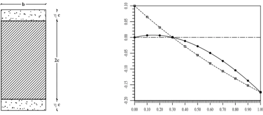
To clarify this point we resort to an academic conceptual problem. Figure 1 (left) shows the rectangular solid section of a beam with height2cand widthb. Letσebe the elastic stress limit of the material. The

section supports the bending mommentMf = 2bc2σe/3, that is the maximum that can be applied without

exceeding the elastic stress limit. We add an upper layer and a lower layer of porous material, both with heightηc(η <<1), and we keep the same value of the bending momment. In these conditions we state the following (trivial) topology optimization problem: find the relative densityρ of the material in the upper and lower layers such that the weight is minimized and the elastic stress limit is not exceeded. It

seems obvious that the exact solution of this problem must beρ= 0.

A quite simple strenght of materials analysis [11] shows that the stress constraint type (16) associated to this problem can be written as

g(ρ) =

η−(3η+ 3η2+η3)ρ

1 + (3η+ 3η2₊_η3₎_ρ

σe≤0. (18)

Figure 1 (right) shows that this constraint is not satisfied for values of the relative density underρ≈1/3. Moreover, the constratint is more severely violated as we get closer to the exact solutionρ= 0! It seems clear that we are facing a situation in which reaching the optimum calls for removing all the material. However, in the vicinity of the optimum (that is for any value ofρslightly greater than0) the constraint is largely violated. Furthermore, its gradient is negative. This is even worse, since any consistent non linear programming algorithm will try to raise the value of the relative density, what precludes convergence to the exact solution of the problem. At the best of times we could only obtain a non global optimum.

If we rewrite constraint (18) in terms of the effective stress (that is, multiplying the above inequality by the relative density) we obtain the alternative stress constraint type (17)

g(ρ) =

η−(3η+ 3η2+η3)ρ

1 + (3η+ 3η2₊_η3₎_ρ

ρ σe ≤0. (19)

(8)

0.00 0.10 0.20 0.30 0.40 0.50 0.60 0.70 0.80 0.90 1.00

-0.20

-0.15

-0.10

-0.05

0.00

0.05

0.10

Figure 1: Layout (left) of an academic conceptual topology optimization problem, and comparison (right) of constraint (18) [] with constraint (19) [•]. (Notes:η=0.1; the constraint is scaled byσ_e.)

important, the gradient is now positive in the vicinity of this point. Therefore, for initial values ofρnot too far from the exact solution (less than 1/6 approximately) any consistent non linear programming algorithm will try to reduce the value of the relative density, what allows to achieve convergence.

This is a critical aspect of these formulations. The challenge is to find a convenient way for limiting the stress, without overestimating the strenght nor trending to fill in regions that should actually be hollowed out. The statement type (17) fulfills partially these requirements. However, it seems to slow down the converge. We have performed a few numerical tests, and this seems to be a quite promising line, although the results are not yet conclusive. A more detailed discussion on this topic can be found in [8].

3.4 The Optimization Problem

Letγmatbe the density of the material. We define the objective function

F(ρρρρρρρρρρρρρρ) =

Z

Ω

ρ1p_γ_mat_d_{Ω =}

nelem

X

e=1

(ρe)

1 p

Z

Ee

γmatdΩ, (20)

wherepis a tuning parameter that can be used to favor a mainly compact (p > 1) or a mainly porous (p <1) distribution of material. In this terms, the topology optimization problem can be written as

Find ρρρρρρρρρρρρρρ={ρρρρρρρρρρρρρρ_e}, e= 1, . . . , nelem that minimizes F(ρρρρρρρρρρρρρρ)

verifying gj(ρρρρρρρρρρρρρρ)≤0, j= 1, . . . , m

0< ρmin≤ρe≤1, e= 1, . . . , nelem

(21)

where the stress constraintsgj (at the corresponding pointsrrrrrrrrrrrrrroj) must be stated accordingly to the

previ-ously exposed concepts, and the stress valuesσσσσσσσσσσσσσσh(rrrrrrrrrrrrrro_j, ρρρρρρρρρρρρρρ)are computed by means of the proposed numer-ical model. Obviously, we can consider displacement constraints too. On the other hand, we introduce a lower limit for the relative density, since the entire hollowing out of some elements could cause a sin-gular stiffness matrix and stall the optimization process. We emphasize that this topology optimization aproach is a kind of sizing optimization from the operational point of view, since the design variables do not modify the shape of the elements. The above stated formulation has been imlemented by following the general methodology [3], and applying the sensitivity analysis techniques [4] and the improved SLP algorithm with quadratic line-search [14] developed by the authors.

(9)

4 Application Examples

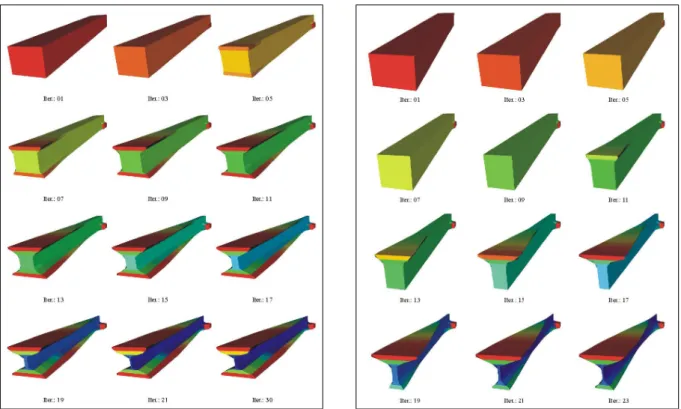
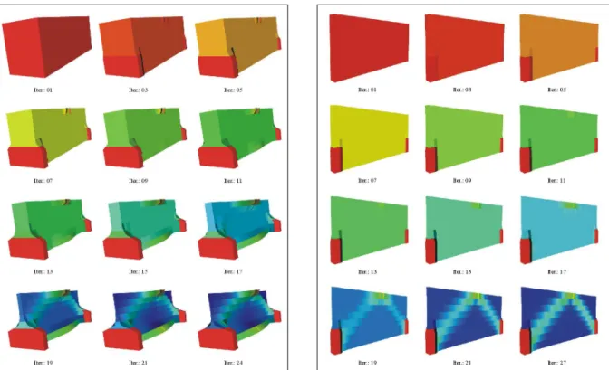
The examples presented below are bidimensional, the width of the structures is constant, and we perform a plane stress analysis. However, the results are represented as 3-D images [8], being the false width pro-portional to the relative density of each element. Figures 2 and 3 show the results for a simply supported structure, with small and large height/length ratio respectively, both for sliding and fixed supports. The domain containing the structure is a prism that bears a concentrated 9000 KN load (vertical, downwards) in the center of the upper side. We analyze half of the structure, because of symmetry. The supports are not optimized. The domain is discretized in 24 times 8 elements (8-node quadrilateral). The mate-rial density isγmat=7650 Kg/m3. Type (16) constraints are imposed at the center of all the elements, in

accordance with the standard NBE EA-95 [15] in terms of the Von Mises reference stressσvm

σvm≤σe; σI ≤2σe; σIII ≥ −2σe. (22)

In figure 2 the domain is 32 m long, 1.5 m high and 1 m wide, and the material is steel with elastic stress limitσe=230000 KN/m2. We notice that the result obtained in the first case is a clear double T shaped

beam with variable section. The width of the wings increases from the supports to the center of the span, where the load is applied. The result obtained in the second case is similar. However, the central section is closer to a T shaped beam. Actually, the lower wing nearly disappears, since the tension due to the bending is balanced with the compression due to the fixed supports. In figure 3 the domain is 32 m long, 12 m high and 1 m wide, and the material is fictitious with elastic stress limitσe=8000 KN/m2. We notice

that the result obtained in the first case is clearly a cable stayed arch. The result obtained in the second case is an arch too, but the tie looses its raison d’ˆetre and it disappears, since the supports are fixed.

(10)

Figure 3: MWSC topology optimization of a simply supported structure, with large height/length ratio, considering sliding (left) and fixed (right) supports. Concentrated load applied in the center of the upper side. (Notes: the supports are not optimized; the entire hollowing out of the elements is not allowed.)

5 Conclusions

In this paper we present a minimum weight with stress constraints (MWSC) approach for topology structural optimization problems. The formulation is derived by introducing minimal modifications to a FEM model for linear elasticity problems with small displacements and small deformations. Although the objective function is simple, as a general rule, this approach leads to more complicated optimiza-tion problems with more computaoptimiza-tional requirements than the maximum stiffness formulaoptimiza-tions, since a large number of highly non-linear constraints must be taken into account to limit the maximum allow-able displacement and stress. In return, the physical meaning of the optimization statement is closer to the engineering point of view, while any kind of constraint can be included and multiple load cases can be considered. The formulation has been implemented in a topology optimization system, and several application examples have been solved. The experience shows that this approach does not require nei-ther stabilization nor penalty techniques to produce acceptable results. The optimized solutions seem to be correct from the engineering point of view and their appearence could be considered closer to the engineering intuition than the traditional truss-like results obtained by the maximum stiffness approach.

Acknowledgements

This work has been partially supported by Grant Number TIC-98-0290 of the SGPICT of the “Ministerio

de Ciencia y Tecnolog´ıa” of the Spanish Government, by Grant Number PGIDT-99MAR11801 of the

SXID of the “Xunta de Galicia”, and by research fellowships of the “Universidad de A Coru˜na” and the “Fundaci´on de la Ingenier´ıa Civil de Galicia”.

(11)

References

[1] L. A. Schmidt, Structural design by systematic synthesis, Proc. of the Second ASCE Conference on

Electronic Computation, Pittsburgh (1960), pp. 105–122.

[2] S. Hernández, Métodos de Diseño Óptimo de Estructuras, Colegio de Ingenieros de Caminos,

Canales y Puertos, Madrid (1990).

[3] F. Navarrina y M. Casteleiro, A general methodologycal analysis for optimum design, Int. J. Num. Meth. Eng., 31, (1991), 85–111.

[4] F. Navarrina, S. L´opez, I. Colominas, E. Bendito y M. Casteleiro, High order shape design

sensi-tivity: A unified approach, Comp. Meth. Appl. Mech. Eng., 188, (2000), 681–696.

[5] M. P. Bendsøe y N. Kikuchi, Generating optimal topologies in structural design using a

homoge-nization method, Comp. Meth. Appl. Mech. Eng., 71, (1988), 197–224.

[6] E. Ramm, S. Schwarz y R. Kemmler, Advances in structural optimization including nonlinear

me-chanics, Proc. of the European Congress on Computational Methods in Applied Sciences and En-gineering (ECCOMAS 2000) (CD-ROM, ISBN: 84-89925-70-4), ECCOMAS, Barcelona (2000).

[7] M. P. Bendsøe, Optimization of structural topology, shape, and material, Springer-Verlag, Heidel-berg (1995).

[8] I. Muiños, Optimización Topológica de Estructuras:Una Formulación de E. F. para la Minimización del Peso con Restricciones en Tensión, Proyecto Técnico, ETSICCP, Universidad de A Coruña (2001).

[9] M. P. Bendsøe, Variable-topology optimization: status and challenges, in W. Wunderlich (Ed.),

Proc. of the European Conference on Computational Mechanics ECCM’99, TUM, Munich (1999).

[10] I. Mui˜nos, I. Colominas, F. Navarrina y M. Casteleiro, Una formulaci´on de m´ınimo peso con

restric-ciones en tensión para la optimización topológica de estructuras, in E. Oñate, F. Zárate, G. Ayala,

S. Botello y M.A. Moreles (Eds.), M´etodos Num´ericos en Ingenier´ıa y Ciencias Aplicadas (ISBN: 84-89925-91-7), CIMNE, Barcelona (2001), pp. 399–408.

[11] F. Navarrina, I. Muiños, I. Colominas y M. Casteleiro, Optimización Topológica de Estructuras:

Una formulaci´on de m´ınimo peso con restricciones en tensi´on, en J. M. Goicolea, C. Mota Soares,

M. Pastor y G. Bugeda (Eds.), M´etodos Num´ericos en Ingenier´ıa V, SEMNI, Barcelona (2002).

[12] T. J. R. Hughes, The Finite Element Method: Linear Static and Dynamic Finite Element Analysis, Dover Publishers, New York (2000).

[13] C. Johnson, Numerical Solution of Partial Differential Equations by the Finite Element Method, Cambridge University Press, New York (1990).

[14] F. Navarrina, R. Tarrech, I. Colominas, G. Mosqueira, J. G´omez-Calvi˜no y M. Casteleiro, An

effi-cient MP algorithm for structural shape optimization problems, in S. Hern´andez y C. A. Brebbia

(Eds.), Computer Aided Optimum Design of Structures VII (ISBN: 1-85312-868-6), WIT Press, Southampton (2001), pp. 247–256.