Hole statistics and superfluid phases in quantum dimer models

Hole statistics and superfluid phases in quantum dimer models

C. A. Lamas,1_{A. Ralko,}2_{M. Oshikawa,}3_{D. Poilblanc,}1_{and P. Pujol}1

1_{Laboratoire de Physique Th´eorique, IRSAMC, CNRS and Universit´e de Toulouse, UPS, F-31062 Toulouse, France} 2_{Institut N´eel, CNRS and Universit´e Joseph Fourier, F-38042 Grenoble, France}

3_{Institute for Solid State Physics, University of Tokyo, Kashiwa 277-8581, Japan} (Received 18 October 2012; published 12 March 2013)

Quantum dimer models (QDMs) arise as low-energy effective models for frustrated magnets. Some of these models have proven successful in generating a scenario for exotic spin liquid phases with deconfined spinons. Doping, i.e., the introduction of mobile holes, has been considered within the QDM framework and partially studied. A fundamental issue is the possible existence of a superconducting phase in such systems and its properties. For this purpose, the question of the statistics of the mobile holes (or “holons”) shall be addressed first. Such issues are studied in detail in this paper for generic doped QDMs defined on the most common two-dimensional lattices (square, triangular, honeycomb, kagome,. . .) and involving general resonant loops. We prove a general “statistical transmutation” symmetry of such doped QDMs by using composite operators of dimers and holes. This exact transformation enables us to define duality equivalence classes (or families) of doped QDMs, and provides the analytic framework to analyze dynamical statistical transmutations. We discuss various possible superconducting phases of the system. In particular, the possibility of an exotic superconducting phase originating from the condensation of (bosonic) charge-eholons is examined. A numerical evidence of such a superconducting phase is presented in the case of the triangular lattice, by introducing a gauge-invariant holon Green’s function. We also make the connection with a Bose-Hubbard model on the kagome lattice which gives rise, as an effective model in the limit of strong interactions, to a doped QDM on the triangular lattice.

DOI:10.1103/PhysRevB.87.104512 PACS number(s): 67.80.bd, 74.20.Mn, 05.30.₋d, 75.10.Kt

I. INTRODUCTION

In 1987 Anderson1 _{suggested that the strange behavior of} cuprate materials between the superconducting dome and the magnetically ordered insulating phase could be described by a resonating valence bond (RVB) state in which preexisting magnetic singlet pairs of the insulating state become charged superconducting pairs when the insulator is doped. Just one year later appeared the first effective model in which the magnetic degrees of freedom are disregarded in favor of the more pertinent singlet degrees of freedom.2 _{This is nothing} but the quantum dimer model (QDM). However, it was soon realized3 _{that the ground state of the undopedS}

=1/2 Heisenberg antiferromagnet on a square lattice exhibits a long-range N´eel order in contrast to the initial expectation based on the RVB picture. Furthermore, the QDM on a square lattice was also found to have only gapped crystalline phases but no evidence of an RVB spin liquid phase in a finite region of the phase diagram.4 _{It is still possible to argue that, even} though the undoped antiferromagnet has the N´eel order, the RVB picture gives a better theoretical starting point once the system is doped with holes. However, it would be natural to ask if the RVB spin liquid phase can be realized in undoped magnetic system with only short-range interaction.

One may expect that magnetic frustration would favor the RVB state over the N´eel phase. Thus, over time, the main interest in the QDM was shifted from the original motivation of the application to high-Tcsuperconductivity, to the effects of frustration. However, clear confirmation of a RVB phase remained elusive for a rather long time. A breakthrough in the study of the QDM was due to Moessner and Sondhi5who showed that a simple QDM defined in the triangular lattice exhibit a disordered phase which, recalling that these dimer models are supposed to be effective models for frustrated

magnets, can be considered as an explicit example of the RVB spin liquid phase. It was also recognized that the RVB spin liquid phase is a topologically ordered phase with a nontrivial topological degeneracy of the ground states.6_{In fact, the RVB} spin liquid phase is essentially identical to theZ2topological phase which was introduced in a completely different context of quantum information processing.7 _{The QDM is generally} not exactly equivalent to an antiferromagnetic Hamiltonian defined in terms of quantum spins. However, the projection from a magnetic system to a QDM was performed successfully in Heisenberg antiferromagnets on frustrated lattices, such as the square lattice with strong enough second and/or third neighbors couplings8,9or the kagome lattice.10These suggest that the QDM may well represent phases without magnetic order in antiferromagnets. In fact, very recently, frustrated Heisenberg antiferromagnets on kagome and other lattices are reported to be in the RVB spin liquid phase (Z2 topological phase) by several authors.11–13

Now that the existence of the RVB spin liquid phase appears to be confirmed in QDMs as well as in antiferromagnets, the issue of superconductivity in doped spin liquids becomes a more pressing question. This issue started in fact to be investigated shortly after the appearance of the QDM.14 Doping of an RVB spin liquid is expected to induce a novel type of elementary excitations called holon. A holon, carrying electric charge e but no spin, appears as a result of fractionalization, namely deconfinement of fractionalized excitations. Indeed, topological degeneracy of the undoped RVB spin liquid is known to be intimately connected to the fractionalization phenomenon.15

issue in this problem is the statistics of the holon. For the holons to condense without forming pairs, they must be bosons. However, it should be noted that transmutation of the statistics16,17 _{is possible. Namely, the statistics of holons} as elementary excitations appearing in the low-energy limit can be different from the statistics assigned to holes in the microscopic model.

In this paper we address the issue of the statistics of holes and its interplay with possible superconducting phases in doped QDMs. In a recent work18_{it was shown that a QDM with} fermionic (at microscopic level) holes is equivalent to another QDM with bosonic holes. Because of the equivalence, the statistics of the holon as a physical elementary excitation must be the same for either representation. This proves the existence of a dynamical statistical transmutation in the system. In this paper we study in more detail the statistical transmutation in QDMs and give a simple and efficient method to obtain the relation between the QDMs with fermionic and bosonic representation of the holes.

In Sec.IIwe introduce a second quantization notation for QDM Hamiltonians and show the gauge symmetry associated with them. In Sec.IIIwe present the composite particle repre-sentation of QDM Hamiltonians which is the key ingredient to show the exact equivalence between a QDM with bosonic and another QDM with fermionic holes. This equivalence is shown for a generic flipping term defined in any kind of lattice. The result, which relies on an orientation prescription of the bonds in the lattice considered, is totally generic and can then be applied to any QDM defined in the most common lattices. The method used here differs considerably from, and has numerous advantages over, the one used in Ref.18where a two-dimensional version of the Jordan-Wigner (JW) trans-formation was used. In Sec.IVwe argue how the modification of the orientation prescription can be interpreted as a simple gauge transformation in the QDM Hamiltonian. We then apply the general result of the statistical transmutation obtained in Sec. III to generic QDM Hamiltonians defined on the square, triangular, hexagonal, and kagome lattices. SectionVis devoted to numerical investigation of four inequivalent QDMs defined on the triangular lattice. In particular, we identify an exotic superconductor phase due to condensation of holons with charge e, measuring numerically the gauge-invariant Green’s function of a single holon. In Sec.VIwe discuss an explicit realization of one of the QDMs discussed in Sec.V. It is obtained as a low-energy strong interaction limit of a Bose-Hubbard model on the kagome lattice. The number of bosons is directly related to the doping, or number of holes, in the resulting QDM on the triangular lattice. SectionVIIis devoted to the discussion of our results. We also include as an appendix the derivation of the statistical transmutation for a generic QDM on the kagome lattice using the Jordan-Wigner transformation. Of course the result is consistent with the one obtained with the composite particle representation obtained in Sec.III, but allows a better understanding of the connection between these two different methods.

II. THE HAMILTONIAN AND ITS GAUGE SYMMETRIES We start with a doped quantum dimer model on a two-dimensional lattice. To fix the ideas, we work here with the

FIG. 1. (Color online) Schematic snapshot of a doped “dimer liquid”. Each site is occupied by either a (single) dimer or a hole (empty site).

Hamiltonian defined on the square lattice but all the arguments remain valid for any two-dimensional lattice. We write the Hamiltonian as

H ₌HJ +HV +Ht (1)

with

HJ=−J + H.C

HV =V +

Ht=−t +

+ + + H.C ,

where the sums are over all the smallest resonant plaquettes on the lattice (for the square lattice these are the squares). In a second quantized formalism we assume that dimer config-urations are created by spatially symmetric dimer operators

b†_i,j and holes are created by bosonic operatorsa_k†(see Fig.1). Then, we can rewrite the Hamiltonian as

HJ = −J

{b_i,j† b†_k,lbj,kbl,i+H.c.}, (2)

HV =V

{b†_i,jb_k,l† bi,jbk,l+b†j,kb †

l,ibj,kbl,i}, (3)

Ht = −t

i

{b†_i,jbj,kak†ai+H.c}. (4) In the last equation, the indices correspond to the labeling of the sites of a square plaquette as in Fig. 2. In our previous conventions, dimer configurations are represented by spatially symmetric operatorsb_i,j† satisfying

[bi,j,b†k,l]=δi,kδj,l+δi,lδj,k, [bi,j,bk,l]=[b†i,j,b † k,l]=0.

(5)

The boson operatora_i†creates a hole in the siteiand satisfies [ai,aj†]=δi,j, [ai,aj]=[a†i,a

†

i

j

l

k

(a)

i

j

_k

(b)

FIG. 2. (Color online) (a) Indexes corresponding to each square plaquette in the HamiltoniansHJandHV. (b) Indexes corresponding to each hopping process inHt.

The operatorsaandbcommute one with each other,

[ai,bj]=[ai†,b † j]=[a

†

i,bj]=0. (7)

We introduce in the model a constraint on the number of dimers and holes which warrants that at each site of the lattice there is either one and only one hole or one and only one dimer arriving to it:

a†_iai+ z_=±eˆ1,±eˆ2

b†_i,i+zbi,i₊z=1. (8)

Of course this constraint implies, among others, that the holes have to be considered as hard-core bosons. It is important to notice that the Hamiltonian has the following U(1) gauge symmetry:

aj →eiξjaj, (9)

bj,k →ei(ξj+ξk)bj,k, (10) where ξi is an angle. This invariance can be exploited to prove the statistical transmutation symmetry in some two-dimensional systems by means of a Jordan-Wigner transfor-mation on the holon operators.18_{In the following we present} an alternative description for the doped QDM using composite operators which allows us to understand in a different way the equivalence between a model with bosonic holes and one with fermionic holes. For doing this, we have first to make a choice of a given orientation prescription for the bonds in the lattice.

III. THE “COMPOSITE” REPRESENTATION FOR THE QDM

A. Composite particles

In order to prove the equivalence between a QDM Hamil-tonian with bosonic holes and another HamilHamil-tonian with fermionic holes, we propose a different formulation for the QDM. This formulation is done in terms of composite particles by defining the operator

Bi,j =bi,jai†a †

j. (11)

This operator destroys a dimer between sitesiandjand creates two holes at the same sites. Let us callHcthe subspace of states that satisfies the constraint(8). For a given state|ψ _∈Hcwe have that_|ψ˜ ₌Bi,j|ψis also a vector inHc.

One can easily notice that the operator Bi,j is invariant under the gauge transformation(9)and(10). This U(1) gauge symmetry was exploited in Ref.14to represent a doped QDM

as a gauge theory coupled to a matter field. More importantly, one can check thatwithin the subspaceHc, the set of operators {Bi,j}form a closed algebra similar to the one of{bi,j}. The Hamiltonian can entirely be written in terms of these Bi,j operators making its gauge invariance manifest. Its precise form is given byH ₌HJ +HV +Htwith

HJ = −J

{B_i,j† B_k,l† Bj,kBl,i+H.c.}, (12)

HV =V

{B_i,j† B_k,l† Bi,jBk,l+Bj,k† B †

l,iBj,kBl,i}, (13)

Ht = −t

i

{B_i,j† Bj,k+H.c.}. (14) It is evident that, within this formulation, the basic building blocks of the model are created by B_i,j† which corresponds to composite particles of charge 2e. Namely, the model is completely defined in terms of the constituent particle with charge 2e. This has several important consequences. In particular, the gauge invariance requires that the energy spectrum of the system on a torus, as a function of the magnetic fluxthrough the “hole” of the torus, is invariant under_→+π/e. (For early discussions on theπ/e-flux periodicity in the QDMs, see Refs.19and20and references therein.) This periodicity corresponds to the unit flux quantum for charge 2eobjects. However, this does not necessarily mean that the physical elementary excitations of the system have minimum charge 2e.15 _{The system can have a topological} order which leads tofractionalization; elementary excitations can have fractions of the charge 2eof the constituent particle of the microscopic Hamiltonian. If the charge-e holons are deconfined as a result of fractionalization, they could condense to form an exotic superconductor.

The apparent contradiction between the periodicity of the energy spectrum inπ/eflux and the expected flux quantization in the unit of 2π/e in the condensate of charge-e holons is resolved by the existence of the topological vortex excitation called vison. Insertion of theπ/eflux corresponds to trapping of a vison. Although the flux periodicity of the ground-state energy does not distinguish an exotic charge-e condensate from the usual superconductor, an experimental detection scheme of the charge-e condensation, based on a “vortex memory effect”, was proposed.21 An actual experiment22 on the high-Tc superconductor did not find such a signature of charge-econdensation. Nevertheless, the exotic superconduc-tivity due to condensation of charge-eobjects is possible in principle, and is an interesting subject to pursue theoretically and experimentally. Later in this paper, we will introduce a quantity which detects a charge-econdensation, and study it numerically in several QDMs.

B. Statistical transmutation symmetry

One of the main advantages of the formulation in terms of composite operators presented above is that one can prove an equivalence between a Hamiltonian where holes are hard-core bosons and another one where the holes are fermions. Let us consider a QDM Hamiltonian with bosonic holes, where their creation and annihilation operatorsa_i†and

annihilated by the set of operators f_i† and fj which now satisfy fermionic anticommutation relations. We then build the respective composite operators:

Bi,j =bi,jai†a †

j, (15)

˜

Bi,j =bi,jfi†f †

j. (16)

As for the operators ˜B, in the rest of the paper all quantities with a tilde correspond to operators and coupling constants of thefermionicrepresentation for the holes. Before proceeding, there is an important statement to make. Again, one can show that within the subspace Hc, both set of operators _{Bi,j} and {_B˜_{i,j} form the same closed algebra of bosonic dimer} operators. Another important point is that the definition of the composite operators in terms of fermions is more subtle because it is necessary to take a prescription for the orientation of the dimers (which determines the order of the fermions in the endpoints of each dimer).

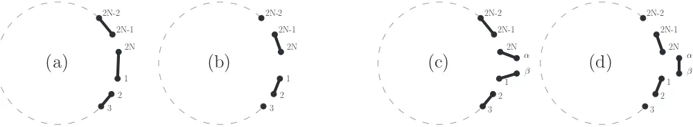
In the following we will call “even prescription” of a given plaquette an ordering prescription for the bonds such that all the bonds are oriented in a clockwise direction or an even number of bonds are oriented anticlockwise. By contrast we call “odd prescription” the prescriptions obtained from the clockwise ordering by flipping an odd number of bonds.

Notice that, since the resonance plaquettes containing N

dimers have necessary 2N bonds, the anticlockwise prescrip-tion (where all bonds are oriented anticlockwise) is always an even prescription.

Theorem. Given a resonant plaquette of arbitrary length with an even prescription for the bonds, then, for the kinetic term of the dimers in the plaquette, we have the equivalence

HJ(J,bosons)↔HJ(−J,fermions). In other words, the res-onance term of dimers in the plaquette is invariant under a simultaneous change of “statistics” of the holes in the system (i.e., bosonic into fermionic or vice versa) and the sign of the dimer resonance loop amplitudeJ.

Proof. Consider a resonance loop containing 2N sites (N

dimers) numbered from 1 to 2N in the clockwise direction as in Figs.3(a)and3(b). The kinetic Hamiltonian for dimers belonging to this loop can be written in terms of bond operators

bi,jas

H_JN ₌J[b₁†_,2b†_3,4b†_5,6. . . b†_{2N−3,2N−3}b†_2N−1,2N]

×[b2,3b4,5. . . b2N₋2,2N₋1b2N,1]+H.c., (17) where the indexNindicates the number of dimers in the loop. Now, we add one dimer (two sites) to the loop, obtaining a resonance loop with N₊1 dimers. In this case, the

Hamiltonian can be written as

H_JN+1 ₌J[b₁†_,2b₃†_,4b†_5,6. . . b†_{2N−3,2N−2}b†_2N−1,2Nb†_α,β] ×[b2,3b4,5. . . b2N₋2,2N₋1b2N,αbβ,1]+H.c. Since all the operators are acting on different bonds they all commute and we can rearrange them in the following way:

H_JN ₌J[b₁†_,2b₃†_{,4· · ·}b₂†_N−3,2N−3b†_2N−1,2N] ×[b2,3b4,5· · · b2N₋2,2N₋1]b2N,1+H.c.,

H_JN+1 ₌J[b₁†_,2b₃†_{,4· · ·} b†_{2N−3,2N−3}b₂†_N−1,2N]

×[b2,3b4,5· · ·b2N₋2,2N₋1]b†α,βb2N,αbβ,1+H.c., or in a compact notation,

H_JN ₌J

⎛ ⎝

N j=1

b₂†_j−1,2j

⎞ ⎠

⎛ ⎝

N₋1 j=1

b2j,2j₊1 ⎞

⎠b2N,1+H.c.,

H_JN+1 ₌J

⎛ ⎝

N j₌1

b₂†_j−1,2j

⎞ ⎠

⎛ ⎝

N₋1 j₌1

b2j,2j+1 ⎞ ⎠b

†

α,βb2N,αbβ,1 +H.c.

Now, we insert on the right of the Hamiltonian the string of operatorsS_Nf ₌2_i=N₁fifi†, where the indexicorresponds to the sites on the resonance loop. This operator acts as the identity operator on the sites belonging to the loop becausefif_i†=1 in the absence of holes. We start with the HamiltonianHN

J :

H_JN ₌H_JNS_Nf ₌J

⎛ ⎝

N j₌1

b₂†_j−1,2j

⎞ ⎠

⎛ ⎝

N−1 j₌1

b2j,2j+1 ⎞ ⎠b2N,1 ×f1f1†· · · f2Nf2†N+H.c.

Now, we move the fermions to the left in order to form the composite operators ˜Bi,j =bi,jfi†f

†

j corresponding to the dimer operators inside the brackets. Commutation of the fermions gives a global sign,

H_JN ₌(−1)ξJ

⎛ ⎝

N j₌1 ˜

B₂†_j−1,2j

⎞ ⎠

⎛ ⎝

N₋1 j₌1

˜

B2j,2j₊1 ⎞ ⎠

×b2N,1f1†f †

2N+H.c.

We can follow exactly the same procedure in the loop withN ₊

1 dimers; the global sign resulting from the commutation of fermion operators to write the products in terms of composite

2N 2N-1 2N-2 1 2 3

(a)

(b)

(c)

(d)

particles is the same as that in theNdimers case. We can write for theN₊1 case,

H_JN+1 ₌(−1)ξJ

⎛ ⎝

N j=1 ˜

B₂†_j−1,2j

⎞ ⎠

⎛ ⎝

N₋1 j=1

˜

B2j,2j₊1 ⎞ ⎠

×b_α,β† b2N,αbβ,1f1†f †

2Nfαfα†fβfβ†+H.c.

Now we can determine the change in the sign ofJ when a dimer is added in the loop. First we commute the operators

f₁†andf₂†_NinH_JN to form the operator ˜B2N,1=b2N,j1f2†Nf † 1. This commutation gives another sign to complete the global phase in the Hamiltonian. Then we can write for theNdimers case

H_JN₌(−1)ξ+1J

⎛ ⎝

N j₌1 ˜

B₂†_j−1,2j

⎞ ⎠ ⎛ ⎝

N₋1 j₌1

˜

B2j,2j₊1 ⎞

⎠B˜2N,1+H.c. In the Hamiltonian corresponding toN₊1 dimers we have to define three composite operators. We have that

b_α,β† b2N,αbβ,1f1†f †

2Nfαfα†fβfβ† =(b†_α,βfβfα)b2N,αbβ,1f1†f

† 2Nfα†f

†

β (18)

=(b†_α,βfβfα)(b2N,αf2†Nf †

α)bβ,1f1†f †

β (19)

= (₋1)(b†_α,βfβfα)(b2N,αf2†Nf †

α)(bβ,1fβ†f † 1) (20) =(−1) ˜B_α,β† B˜2N,αB˜β,1. (21) Finally, the Hamiltonian corresponding toN₊1 dimers reads

H_JN+1₌(−1)ξ+1J

⎛ ⎝

N j=1 ˜

B₂†_j−1,2j

⎞ ⎠

⎛ ⎝

N₋1 j=1

˜

B2j,2j₊1 ⎞ ⎠

×B˜_α,β† B˜2N,αB˜β,1+H.c.

We have proved by induction that, if for aN dimers loop, the kinetic term acquires a given sign when the Hamiltonian is written in terms of fermionic composite particles, then the kinetic amplitude corresponding toN₊1 dimers acquires the same sign. To complete this mathematical induction proof we need check that the statement holds for the lowest value ofN. The smallest possible resonance loop is given by a loop with only two dimers. It is easy to check that in this case

H_J2₌J b†_1,2b†_3,4b2,3b4,1+H.c.

=J b†_1,2b†_3,4b2,3b4,1f1f1†f2f2†f3f3†f4f4†+H.c. =(−1)JB˜₁†_,2B˜₃†_,4B˜2,3B˜4,1+H.c.

Then we have proved that the kinetic term for a resonance loop of arbitrary length oriented in a clockwise direction, the amplitudeJ in the Hamiltonian written using dimer operators

bi,j, changes to−J when we write the Hamiltonian in terms of fermionic composite operators ˜Bi,j. A trivial verification shows that the amplitude remains unchanged when we write the Hamiltonian in terms of bosonic operatorsBi,j =bi,jai†a

† j. The result above can be rewritten in the more appealing way:

HJ(J,B˜)≡HJ(−J,B). (22)

The proof can easily be extended to the potential termHV. In this case it is easy to see that the bosonic and fermionic versions give the same sign in the amplitudeV,

HV(V ,B˜)≡HV(V ,B). (23)

The equivalence proved above is valid for any even prescription on the plaquette. Starting from the clockwise prescription where the results above have been proved, if we flip two bonds this induces the commutation of two fermionic operators and the sign remains unchanged. But if we flip an odd number of loops we must commute an odd number of extra fermionic commutations in order to form the composite operators. These permutations give an extra sign in the Hamiltonian. Then it is easy to prove the following corollary:

Corollary 1. Given a resonant plaquette of arbitrary length with an odd prescription for the bonds, then, for the kinetic energy of the dimers in the plaquette, we have the equivalence

HJ(J,bosons)↔HJ(J,fermions).

The equivalence in the potential term does not change if we take an odd or even prescription. Using this property of the potential term and Corollary 1 we can derive the following corollary.

Corollary 2. Note that we have actually proved that, if in a given lattice we can take an even prescription for all the plaquettes involved in the Hamiltonian, then the equivalence

H(J,V ,bosons)_≡H(₋J,V ,fermions) (24)

is valid for the Hamiltonian in the complete lattice, whereas if we can take an odd prescription for all the plaquettes in the Hamiltonian, we have the equivalence

H(J,V ,bosons)_≡H(J,V ,fermions). (25)

In order to complete the panorama for the doped QDM we study the fermionic and bosonic representation of the HamiltonianHtcorresponding to the hopping of holes.

Consider three nearest-neighbors sites of the lattice as in Fig.2(b). In terms of bosonic holes and dimer operators we can write a general hopping term as

h(_i,j,kt) ₌b_i,j† bj,ka†kai (26) if there is no hole in the intermediate sitej we can add on the right the identity asajaj†=1. We then obtain

h(_i,j,kt) _{= −}t b†_i,jbj,kak†aiajaj† (27) = −t(b†_i,jajai)(bj,kaj†a

†

k) (28)

= −t B_i,j† Bj,k. (29) In the bosonic case we do not need to worry about the prescription in the lattice but it is important when we study the fermionic description. In this case we take the prescription

i_→j _→k. Starting from the Hamiltonian

˜

h(_i,j,kt) ₌b_i,j† bj,kfk†fi (30) we insert on the right the operatorsfjfj†=1,

˜

h(_i,j,kt) _{= −}t b†_i,jbj,kfk†fifjfj† (31) = −t(b†_i,jfjfi)(bj,kfj†f

†

k) (32)

(a)

(b)

(c)

(d)

FIG. 4. (Color online) Bond prescriptions on the square (a), triangular (b), honeycomb (c), and kagome (d) lattices. Light-blue plaquettes have an even prescription while the green plaquette has an odd prescription.

Using the prescription i_→j _→k, the amplitude in the hopping term for the holes is the same if we use the fermionic or bosonic versions of the composite operators. Flipping two arrows we have the prescription k_→j _→i. It is a simple matter to see that with this prescription the hopping amplitude is also the same for the two cases.

Then, the hopping of the holes written in terms of bosonic and fermionic composite operators have the same amplitude

t, provided that we use one of the two prescriptions satisfying that the intermediate site has one incoming and one outgoing arrow. If we take thisi_→j _→kprescription in all the sites of the lattice the arrows follow a sort of Kirchhoff’s first rule; see Figs.4(a),4(b), and4(d). We will call this kind of prescription “zero-current” prescriptions. Of course it is only possible to satisfy this prescription in all the sites if the coordination number of the lattice is even. An example where this is not possible is the Honeycomb lattice (withz₌3). In this lattice it turns out that it is not possible to take a prescription with the same number of incoming and outgoing arrows in each site; see Fig.4(c).

IV. QDM CLASSIFICATION FOR DIFFERENT LATTICES A. On the choice of the bond orientation prescription As we saw in the last section, in order to prove the equivalence between Hamiltonians built with bosonic and fermionic operators, one needs a bond orientation prescription for the fermionic case. Of course, this prescription is totally

arbitrary and before proceeding it is important to clarify the issue of a different choice of prescription. Let us imagine a generic lattice for which we have chosen two different prescriptions,AandB. To clarify the ideas, imagine that the orientation of all the bonds in prescription B are the same that in prescription A, except for one single bond, which is connecting pointsi andj. Then, starting from a bosonic Hamiltonian, by doing the transmutation, we end up with two different HamiltoniansHAandHBwhich have the same signs for all the flipping and hopping terms except for the ones that contain the bondij. Let us illustrate this with the following example: consider the square lattice in which prescriptionAis the one given in Fig.4. Then, imagine a prescriptionBwhere only the arrow between sitesi andj is reversed, as shown in Fig.5. Starting from the same bosonic Hamiltonian, after the statistical transmutation, we get the HamiltoniansHAand

HB. What is the difference betweenHAandHB? They have the same signs for all the flipping terms, except the the ones of plaquettesαandβ, which are the only two containing this reversed bond. Also, all hopping terms are the same except those containing the linkij.

Although one could naively think that these two re-sulting Hamiltonians are not equivalent, in fact they are, as can be easily seen by performing the following gauge transformation:

A

i j

α

β

i j

B

α

β

FIG. 5. (Color online) The change of prescription corresponding to reversing the orientation of one single bond (ij in the figure) corresponds to a gauge transformation where only configurations containing a dimer in theijbond have their sign changed. This in turn has the effect of reversing the sign of the flipping and hopping terms containing the bondij, as, for example, the flipping of plaquettesα andβ.

Most generally, it is easy to convince oneself that different choices of prescriptions give rise to apparently different Hamiltonians which in fact are equivalent under a certain gauge transformation. We are now going to consider each lattice in detail and justify for each of them the choice of prescription we have made.

B. Square lattice

For the square lattice, we consider the prescription given in Fig.4(a). Using this prescription, the hopping amplitude (t) remains equal for the bosonic and fermionic representationB

and ˜B. On the other hand, the kinetic amplitude corresponding to dimers (Jα) changes its sign if an even prescription is induced in the plaquette of lengthα. In Fig.4the plaquettes of lowest order are shown. Light-blue areas correspond to even prescriptions induced in the plaquettes while green areas correspond to odd prescriptions. The relative sign between the couplings in the fermionic and bosonic representations corresponding to the eight smallest plaquettes are presented in TableI.

TABLE I. Values of ˜Jα/Jαcorresponding to the lowest orders of the resonant plaquettes on the square lattice.

N Loop J /_J/t˜˜t

2 -1

3 1

4

-1

-1

-1

5

1

1

1

TABLE II. Values of ˜Jα/Jαcorresponding to the lowest orders of the resonant plaquettes on the triangular lattice.

N Loop J/_J/t˜t˜

2

-1 -1

-1

3

1

1

-1

C. Triangular lattice

For the triangular lattice, as in the square case, the coordination number is even and we can take a “zero-current” prescription as shown in Fig.4(b). Then the hopping amplitudes for bosonic and fermionic holons have the same sign. Again, the change in the sign when we change from a bosonic representation of the holes to a fermionic one is determined by the parity of each flipping term. In TableII we show the results for flipping loops containing up to three dimers.

D. Honeycomb lattice

The case of the Honeycomb lattice is more subtle. The coordination number in this lattice is z₌3 and it is not possible to take a “zero-current” prescription. Therefore, it is not possible to find a prescription in which all the hopping terms would remain the same after the transmutation. We then use the prescription of Fig. 4(c) in which all the hopping amplitudes for the holes change the sign when we change to the fermionic representation of the operators (˜tn= −tn).

The relative signs between the ratios ˜J /t˜ and J /t are presented in Table III for plaquettes of three, five, and six dimers.

E. Kagome lattice

For the kagome lattice, we have chosen the prescription depicted in Fig.4(d). All the possible allowed flipping terms

TABLE III. Values of ˜Jα/Jαcorresponding to the lowest orders of the resonant plaquettes on the honeycomb lattice.

N Loop J /_J/t˜˜t

3 -1

5 -1

up to 12 bonds are depicted in TableVIof the Appendix. Is it interesting to note that these loops are all, without exception, even. This feature is not specific to loops of short lengths and one can convince oneself that all allowed flipping loops of arbitrary length are even. Moreover, our prescription choice is such that the hopping terms within one triangle remain invariant under the statistical transmutation. From this, one can conclude that a Hamiltonian with flipping terms{Jl}and bosonic holes is equivalent to a Hamiltonian with fermionic holes and with the signs of all flipping terms reversed_{−Jl}.

One last remark one can make about the kagome lattice relies on its intrinsic flexibility. Take any triangle of it and change the orientation of the three bonds belonging to that triangle only. It is easy to see that with the new prescription all the hopping terms, including those belonging to the chosen triangle, do not change signs. However, the flipping terms containing one (and only one) bond belonging to that triangle will change their signs, i.e., these flipping terms in the transmutated Hamiltonian have the same sign as in the bosonic model. What this means is that, in contrast to the other lattice studied here, it is possible on the kagome lattice to build gauge transformations which leave invariant the sign of all hopping amplitudes while changing the sign of “some” flipping terms (even locally).

F. Example of application of the “statistical transmutation” symmetry

To illustrate the power and extent of our results, we concentrate on a couple of concrete examples taken on the square and triangular lattices, respectively. Let us consider the QDM defined on the square lattice with only two and three dimer flipping terms. These terms correspond to the first and second row of TableI. Its sibling model can be defined on the triangular lattice by just considering the terms with N₌2 and only the second of the terms withN ₌3 in TableII. In principle we would have 16 inequivalent Hamiltonians in each case. However, our statistical transmutation result tells us that the number of inequivalent Hamiltonians is smaller. Indeed, we find only eight inequivalent Hamiltonians for the case of the triangular lattice, which we dubbed Iσ, IIσ, IIIσ, and IVσ, where σ _{= ±} corresponds to the sign of the hopping term. From these eight classes only four classes are inequivalent for the case of the square lattice. The smaller number of equivalence classes in the latter case is due to to the equivalence

t _{↔ −}t which is valid for the square lattice but not for the triangular lattice.18The result is summarized in TableIV.

G. Transformation of assisted terms

When a QDM is regarded as a low-energy effective model of frustrated antiferromagnets, it is important to see if other kinds of term, apart from those already mentioned here, arise in the effective QDM Hamiltonians. Examples of derivation of the QDM Hamiltonian arising from microscopic Heisenberg models can be found in Ref. 9 for the square lattice with second- and third-neighbor couplings and in Ref.10for the kagome lattice. In these QDMs appears a third kind of diagonal or off-diagonal terms, which are dubbed assisted terms. Let us now discuss these assisted terms in our framework. An example of such terms is given in the last row of Table I

TABLE IV. Classification for the doped QDM with resonant plaquettes of length 4 and 6. For the square lattice the families I₊ and I₋are equivalent (idemfamilies II, III, and IV). For the triangular latticeJ4corresponds to the three resonant plaquettes corresponding toN=2 in TableIIwhereasJ6corresponds to the second row of N₌3 in the same table. The last two columns show the references where such models have been studied (forJ6=0) on square () and triangular (_△) lattices.

Statistics J4 J6 t Family Refs. () Refs. (△) Bosons + + + I₊ 23,24,25,26 18,24,26

Bosons _{+ + −} I₋ 23,25 18

Bosons _{+ − +} II₊

Bosons + − − II₋

Bosons _{− + +} III₊ 23 18

Bosons − + − III₋ 23 18

Bosons _{− − +} IV₊

Bosons − − − IV₋

Fermions _{+ + +} III₊ 23 18

Fermions _{+ + −} III₋ 23 18

Fermions + − + IV₊

Fermions _{+ − −} IV₋

Fermions − + + I₊ 23 18

Fermions _{− + −} I₋ 23 18

Fermions − − + II₊

Fermions _{− − −} II₋

in Ref.9. They consist of diagonal or off-diagonal terms of the kind of the HV andHJ in Hamiltonian (1) but subject to the condition that a third dimer is sitting in another given neighboring bond. Such kind of term can be written as, for example,

[b†_i,jb_k,l† bj,kbl,i+H.c.][b†m,nbm,n], (34) whose effect is to flip two parallel dimers sitting in the plaquettei,j,k,lprovided that there is one dimer sitting in the plaquettem,n. By extending the arguments developed above, one can show that under the statistical transmutation, this kind of term transforms in the very same way as the corresponding nonassisted term. For example, the term written above would transform in the same way as the term

b†_i,jb_k,l† bj,kbl,i+H.c. (35) This is simply due to the fact that assisted terms can be written as the product of traditional diagonal or off-diagonal operators which we know already how they transform and projectors which are written in terms of dimer density operators which are invariant under the statistical transmutation.

V. NUMERICAL INVESTIGATION OF QDMs ON THE TRIANGULAR LATTICE A. Summary of phase diagrams in Ref.18

0 0.1 0.2 0.3 0.4 0 0.5 1

0 0.1 0.2

0 0.5 1

(a)

(b)

(c)

(d)

x

x

C

ry

st

a

l

Z2

li

q

u

id

C

ry

st

a

l

Z2

li

q

u

id

V

|J|

V

|J|

Phase Separation

Superfluid

Superfluid

F

e

rm

io

n

ic

p

h

a

se

Phase Separation

“Complex” phase Supersolid

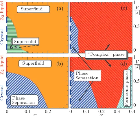
FIG. 6. (Color online) Qualitative phase diagrams of four in-equivalent doped QDM’s on the triangular lattice versus doping (x) andV /_|J_|for fixedt /J ₌0.5, from Ref.18. All the models have only flipping terms corresponding to N=2 in TableII. Case (a) corresponds to positiveJ andt and bosonic holes, (b) is obtained from (a) by changing the sign of the hopping termt, (c) is obtained from (a) by changing the bosons to fermions, and (d) is obtained from (b) by changing the bosons to fermions.

of the results obtained in Ref.18. Considering only flipping terms J ₌J4 involving the shortest loops corresponding to

N ₌2 in TableIIa topological (Z2) liquid can be stabilized at zero doping5,27 (the sign ofJ is irrelevant forx ₌0). At finite doping, four nonequivalent families of Hamiltonians can be constructed depending on the signs oft andJ. Note that changing the bare statistics of the holons does not introduce a new class of Hamiltonian since this is equivalent to change the sign of J as seen in the previous sections. In other words, one can equivalently choose to work in the bosonic or fermionic representations. In contrast, the actual statistics of the elementary excitations has to be studied numerically. One can use, e.g., the method developed in Ref.23which consists of investigating the node content of the wave functions.

The phase diagrams of the four families of models obtained in Ref.18are reproduced in Fig.6for convenience. At zero doping (where the four models merge into the same x₌0 limit) there are two (insulating) phases, (i) a six-site cell valence-bond crystal (VBC) for 0V /_|J_|0.7 and (ii) a topological Z2 dimer-liquid above. At finite doping, family (a) in Fig. 6 is the only unfrustrated case and was studied using the Green’s function Monte Carlo (GFMC) methods in Ref. 24. In this model bare holons are bosonic and remain representative of the physical excitations in the entire region of the phase diagram, as happens also in the Perron-Frobenius square lattice version, studied in Ref.23. The situation is even more interesting whenJ is changed into−J, or equivalently, bosons are changed into fermions [families (c) and (d) in Fig. 6]. Finally, changing the signs of both J andt of the unfrustrated model (a) leads to the complex case (d). Note that the PS regions are further increased atV <0 so we restrict here only toV >0.

WhenJ becomes comparable to the holon average kinetic energy (of orderxt) holons may be macroscopically expelled from the dimer fluctuating background, in order to minimize the dimer resonance energy. The question ofphase separation (PS), i.e., the possibility for the system to spontaneously undergo a macroscopic segregation into two phases with different hole concentrations, was considered in Ref. 18. In order to perform a Maxwell construction one can defines(x)= [e(x)₋e(0)]/x, wheree(x) is the energy per site at doping

x₌nh/N (nh is the number of holons in the system andN the number of sites). In the case of PS, the energy presents a change of curvature at a critical dopingxccorresponding to the minimum ofs(x) as a function ofx. The fact that the local curvature ofe(x) atx₌0 is negative then implies that the two separated phases will havex ₌xc andx=0 (the undoped insulator) hole concentrations. This study revealed that all frus-trated [(b)–(d)] models show a finite PS region [shown in blue in Figs.6(b)–6(d)] at low doping. The extension vsV /_|J_|of this region seems to coincide with thex ₌0 VBC. In contrast, the nonfrustrated (a) model does not show phase separation atV >0 (as already seen in GFMC simulations) but, rather, shows a homogeneous region at finite doping where VBC order survives. Because of the coexisting nonzero superfluid order [U(1) symmetry breaking, see below], this phase can be viewed as a “supersolid” (SS). Here supersolidity involves hole pairingin the vicinity of a (insulating) VBC phase (and in the absence of PS), as also found in thefrustrateddoped QDM on the square lattice23or in doped frustrated spin-1/2 quantum magnets.28

Another important quantity used in Ref. 18 is the sign operator defined in Ref. 23 which provides a quantitative analysis of the nodal structure of the wave function and hence gives insights about the statistical nature of the holons, i.e., whether they truly behave as bosons or fermions. Such an analysis clearly showed that the GS of models (a) and (b) have the same nodal structure as a superfluid. For models (c) and (d), we dubbed a “complex phase” as the statistics of dressed excitations does not correspond solely to bosons or fermions. Family (d) also shows, in addition, an interesting fermion reconstruction at large doping, which we call the “fermionic phase”. In this work we have extended the study of the nodal structure for larger values of the doping than the ones of Fig.6. Our results clearly show that forx0.6 the elementary excitation behaves as bosons for the four models. This means in particular that in model (d) a dynamical statistical transmutation took place in which each Fermion bound to a vison in order to form a boson. As we show below, this result has important consequences in the nature of the superfluid phases that we find for those values of the doping.

as already discussed in Sec.III A, theπ/(2e)-flux periodicity is a generic feature of doped QDMs and does not rule out the possibility of condensation of deconfined charge-eholons. Next, we will characterize more thoroughly the nature of the superfluid phases, by introducing a gauge-invariant holon Green’s function to distinguish the charge-econdensation from the usual charge-2econdensation.

B. New correlations to explore the nature of the superfluid phases

In order to understand the nature of the superfluid phases the effective charge of the quasiparticles that condensate have to be determined—either charge-eor charge-2equasiparticles. This is related to the mechanism that leads to the spontaneous breaking of the U(1) symmetry expected in a superfluid. As a first attempt, one could naively use the correlation function

a_k†aj, but it is not compatible with the constraint (8). In other words, it is not gauge invariant and thus this correlation function is zero. To satisfy the constraint, or equivalently the gauge invariance, we need to write correlations in terms of operatorsB. As the hopping of holes can be written in terms of operatorsB we can move one of the holes between two distant sites by applying a string ofB†B’s.

1. Gauge invariant holon Green’s function

In the subspace where the constraint is satisfied pairs of holons operatorsaiai†acting on sites without holes are equal to the identity. Then the holon Green’s function we want to calculate is given by

G(_i,jb) ₌

n

a_i†S_j,i(n)aj

, (36)

whereSj,i(n) =b †

j,n1bn1,n2b

†

n2,n3bn3,n4. . . b

†

nN−1,nNbnN,iis a string operator between the sitesiandj following the pathn. The label (b) indicates that the holes are taken as bosons. Similarly, the fermionic version of the Green’s function is written as

G(_i,jf) ₌

n

f_i†Sj,i(n)fj

. (37)

Note that, since there are many ways of moving a hole between two sites, the gauge invariance alone does not uniquely determine the definition of the holon Green’s function. Here we adopt the definition with a sum over all possible strings (labeled by n) connecting the two sites i and j, with the same coefficient. This definition appears most natural to us, as well as in numerical implementation. We expect that other definitions with some restrictions on strings would also work as an order parameter. However, the present definition looks advantageous in numerical calculations, since it can efficiently detect the holon condensation with the summation over all possible strings. Notice that, because of the constraint on the dimers, the paths are necessary self-avoiding.

Using a complete basis of dimer/hole configurations the correlations can be rewritten as

G(_i,jb) ₌

n

α,β

ψ_|α β_|ψ α_|a†_i S_j,i(n) aj|β, (38)

G(_i,jf) ₌

n

α,β

ψ_|α β_|ψ α_|f_i†S_j,i(n)fj|β. (39)

The holon Green’s function can be also written in terms of the composite operators only,

G(_i,jb)₌ {n_}

B_N†_−1,NBN,i. . . B2†,3B3,4B1†,jB1,2, (40)

G(_i,jf)₌ {n_}

˜

B_N†_−1,NB˜N,i. . .B˜2†,3B˜3,4B˜1†,jB˜1,2, (41)

where the sum is over all possible paths between sites i

andj. One can use this representation to show that the two correlations are in fact equal, up to an irrelevant sign. In other words, we have

G(_i,jb) _{= ±}G(_i,jf), (42) where the relative sign depends only on therelativedistance between i and j. Off-diagonal long-range order of Gi,j is a fingerprint of the spontaneous breaking of the U(1) gauge symmetry (associated to charge conservation). It also implies that the condensing quasiparticles have charge e. It is also interesting to observe that at large doping, this Green’s function must necessarily have an exponential decay (see below). Indeed, the Green’s function for being nonzero needs at least one path in which dimers are present all along it (the string). For a large concentration of holesx_→1 it is more and more unlikely to find a path with dimers on it so that the Green’s functionGi,jshould roughly decay as (1−x)LwhereLis the distance between pointsiandj.

Another observable which can detect the charge-e conden-sation is

Fi,j = a†i S (n) j,i a

† j

, (43)

when a symmetry-breaking ground state (when it occurs) formed by superposition over different dimer-number sectors is used. Roughly speaking, this corresponds to the square of the expectation value of a single hole creation operator a†in the ground state, defined in a gauge-invariant manner. Such an expression is however less convenient to compute numerically in finite-size systems and will not be used.

The scenario of Bose condensation of polarized spinons (the holons in our current formulation) under an applied magnetic field advocated in Ref.24implicitly implies long-range order of Gij. We wish here to substantiate such a scenario by an explicit computation of this correlation function.

2. Hole pair correlations

IfGi,jis short ranged, there is no condensation of charge-e holons. However, spontaneous U(1) symmetry breaking and, hence, superfluidity can still occur provided the (hole) pair-pair correlation,

Pi,j,k,l = Bi,jBk,l† , (44)

TABLE V. Classification of the possible phases, including various superfluid (SF) phases, that may occur in doped QDM’s on the triangular lattice. Such phases can be distinguished from the sign of the compressibilityκ, the long-distance properties (“SR” means short-range, “LR” means long-range) of various correlations, or the effective charge deduced from periodicity of the GS energy versus a magnetic flux inserted through a torus. sgn_Band sgn_Fwere defined in Ref.23to analyze the node content of the GS wave function.

Observables→

Phases↓ κ b

†

i,jbi,jb

†

k,lbk,l a

†

ka

†

laiaj a

†

iSi,jaj sgnB sgnF Flux periodicity

PS <0

VBC >0 LR SR SR 2e

SS >0 LR LR SR 1 0 2e

2e-SF >0 SR LR SR 0<sgnB<1 0<sgnF <1 2e

e-SF >0 SR LR (weak) LR 1 0 2e

Bose liquid >0 SR SR SR 1 0 2e

Fermi liquid >0 SR SR SR 0 1 2e

“Complex” phase >0 SR SR SR 0<sgnB<1 0<sgnF <1 2e

operator in a complicated manner. Namely,

a_i†

n

S_k,i(n)ak)(a_j†

n′

S_l,j(n′) al

+

a_i†

n

Sl,i(n) al)(a † j

n′

Sk,j(n′) ak

= Bi,jBk,l† + {loop terms}, (45) where the first part of the right-hand side is obtained from a “closure relation” involving all pairs of “retraceable” strings

n′₌n¯, i.e.,

n

S_k,i(n)S_l,j( ¯n)₊S_l,i(n)S_k,j( ¯n)

=bijbkl†, (46)

and the rest corresponds to pair hopping dressed with extra loop fluctuations. The proof for Eq.(46)is not straightforward but the reader may be easily convinced of this result by drawing the paths for some examples. This suggests that it is physically meaningful to write the pair correlations as

Pij kl=GikGj l+GilGj k,+Pij klc , (47)

where the first two terms can be viewed as the “mean-field” contribution and P_{ij kl}c stands for the “connected” part in which we remove all the processes involving compositions of single holon hoppings. In particular, both sides scale like

x2 _{or (1}

−x)2_{, respectively, in the limit x}

→0 or x _→1. Therefore it is convenient to normalize Pij kl by x2(1−x)2 and Gij by x(1−x). Equation (47) shows that LRO in the holon Green’s function Gik→G_∞, characteristic of the charge-esuperfluid, will inevitably induce LRO in the pair-pair correlation,P _∼G2

∞. In contrast, the conventional, charge-2e

superfluid is defined by LRO in the connected parttogether with the short-ranged holon Green’s function.

3. Dimer-dimer correlations

We finish by recalling that the dimer-dimer correlations are expressed in terms of the dimer number operatorsb†_i,jbi,j as

Ni,j,k,l= b†i,jbi,jbk,l† bk,l, (48) where sitesiandjon one hand, andkandlon the other hand, are nearest-neighbor sites. Long-range order in this correlation

function is characteristic of VBC order. The wave vector at which the associated structure factor diverges defines the VBC wave vector.

In principle, one can use the new correlations Gi,j and

Pi,j,k,lto refine the previous phase diagrams (Ni,j,k,lwas used in previous work to determine the VBC and SS regions). To ease the analysis of the numerical results of the doped QDM’s, a classification of the various possible phases based on simple considerations is provided in TableV.

We note that there is no phase where there is a charge-e

condensation simultaneously with a dimer long-range order (“LR” for both b_i,j† bi,jbk,l† bk,land a†iSi,jaj.) This is because existence of the dimer long-range order leads to confinement of holons.

C. Numerical results

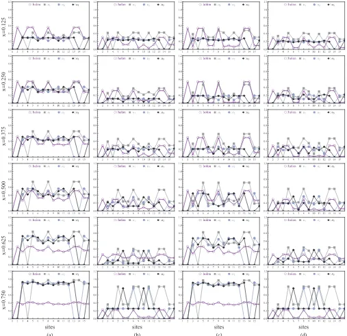
In Fig.8 are displayed both the holon Green’s functions [Eqs.(36)and(37)] and thesquare rootof the pair-pair correla-tions [Eq.(44)] computed by numerical exact diagonalization on a 16-site triangular cluster, varying the hole density from

x₌0.125 (low hole concentration) to x₌0.75 (low dimer concentration), from top to bottom. For convenience, both

1 2 3 4

5 6 7 8

9 10 11 12

13 14 15 16

FIG. 8. (Color online) Holon Green’s function (open circles) andsquare rootof the absolute value of the pair-pair correlations (filled symbols) for parametersV =0.3,_|J| =1.0, and_|t| =0.5, at various densities ranging fromx=0.125 tox=0.75 (2 to 12 holons on 16 sites) and for the four classes (a)–(d) of models defined in the caption of Fig.6. The pair-pair correlationPi,j,k,lis defined by a reference bond orientationτj ₋ τi₌ uαand the orientation of the final bondτl₋ τk₌ uβ. In our case, we choseuα ₌ u1and we consider three cases foruβ:

u1(filled squares),u2(filled circles), andu3(filled diamonds)—see Fig.7. the Green’s functions and the square root of the pair-pair correlations are normalized by x(1−x) to be able to use the same scale for all densities. The four Hamiltonian classes defined previously (see, e.g., the caption of Fig.6) are depicted in parallel panels (a)–(d), respectively. For all of them. we chose the parameters V ₌0.3, _|J_{| =}1.0, and _|t_{| =}0.5 for which, at holon density x₌0.25, the system is either in a superfluid phase [Figs. 6(a) and 6(b)] or in the “complex” phase [Figs.6(c)and6(d)], depending on the QDM class.

Let us first discuss the data at the lowest hole densities

maybe for model (c) around x _∼0.5. On the other hand, the pair-pair correlations, for which the reference link is in the u1 direction, show convergence with bond separation to a uniform value for model (a) in all relative directions of the two bonds, while these correlations are strongly reduced for directions differing from that of the reference bond in the other models. Hence our data are clearly compatible with model (a) being in the charge-esuperfluid phase described in Table V, unambiguously revealing strong signals simulta-neously in the holon Green’s function and the pair-pair correlation. Note that we also checked that the dimer-dimer correlations (not presented here) remain SR in model (a) hence reinforcing the previous claim. The behavior of the other models at low to moderate doping is less clear, with quite smaller amplitudes of Gij and Pij kl at the largest available distances. We can, however, recognize a possible 2e-superfluid phase in model (c) after the phase separation zone and up to values ofx_≃0.2.

While increasing holon density, fromx₌0.5 tox ₌0.75, we observe that the data for the bosonic and fermonic models become identical, both for t >0 or t <0. This can be understood by the fact that the (bosonic) dimers become then the relevant entities instead of the holes. This implies, in particular, that statistical transmutation or pairing must occur for increasing x for the models where fermionic statistics is expected at small x [models (c) and (d)]. This is indeed confirmed by the analysis of the nodal structure of the wave functions that we performed for x ₌0.625. In this sense the complex phase found in model (c) is probably the region in which fermions bound to visons and transmute, in order to resemble the bosonic excitations of model (a). Note also that charge-esuperfluidity seems to occur atx ₌0.625 in models (a) and (c) (which seems equivalent for this doping).

However, at largerxcorresponding to a dilute gas of dimers one expects to eventually recover a charge 2esuperfluid via a continuous (second order) or discontinuous (first order) phase transition. This seems to occur already forx ₌0.75 for models (b) and (d), for which only the pair-pair correlations are sizable at the largest distances. We have checked that for a lower dimer density of 1₋x_∼0.1 Gij is short range for allmodels as reported in Fig.9. In the limit of a very dilute gas of dimers, pairing between dimers because of the kinetic termJ is also a possibility. This could result in either phase separation or in a homogeneous phase in which bothGij andPij kl are short ranged but which is nevertheless superfluid, of coherent dimer pairs of charge 4e. We have checked that there is no phase separation in any of the four models at those large values ofx. We have also looked at the energy difference between two and one dimers and found that pairing is indeed favored in models (b) and (d) which may explain the drop of thePij kl in Fig.9 forx 0.9.

Based on Figs.6,8, and9, we have extracted the qualitative phase diagrams for the four models at fixedV /_|J_{| =}0.3 and

t /_|J_{| =}0.5 as a function of doping x. They are depicted in Fig.10. Charge-esuperfluidity seems to occur in all models, with the largest occurrence in model (a). For intermediate doping, models (b) and (d) seem to present short-range correlations for both one- and two-particle Green’s functions. This behavior suggests an uncondensed phase which in the

case of model (d) would correspond to a Fermi-liquid state. Since elementary excitations in model (b) are bosonic the presence of an uncondensed phase points toward an exotic Bose-liquid state, although this statement should require a more detailed study (using clusters of a much bigger size) which is beyond the scope of the present paper. For largex, all models exhibit a charge-2esuperfluid phase as expected, followed by a charge-4e superfluid phase in models (b) and (d) due to dimer pairing.

VI. CONNECTION TO BOSE-HUBBARD MODELS We finish this work by discussing the connection to Bose-Hubbard-like models which do not containa priorithe ice-rule constraint. However, the physics of the doped QDM can emerge naturally when some form of large repulsion between the itinerant bosons is considered, hence providing emergence of fractionalized excitations.30

In Ref. 30 was introduced a simple model of hard-core bosons hopping (t) on a kagome lattice with a boson repulsion

Vfavoring the smallest number of bosons in each hexagon,

H _{= −}t

i,j

(d_i†dj +didj†)+V

(n)2, (49)

where d_i† creates a boson on site i and n=6_i=1d_i†di is the number of bosons in a hexagonal plaquette. When the boson density isρ₌1/2 a largeV/tstabilizes an insulating phase whose quantum dynamics is described by a generalized QDM on the triangular lattice with exactly three dimers per site. The insulating phase is aZ2 topological liquid. When

t <0 the model is not frustrated and can be studied with QMC: the superfluid-insulator transition was argued to be a novel nonconventionalfractional critical point.30

To make the connection with some of our doped QDM’s we shall assume here that the microscopicd bosons have charge −2eand their density is set toρ₌1₆(1−x/2),x _≪1. In that case, as shown in Fig.11, forV/t→ ∞the lowest-energy configuration space (E₌N V/3) is given by all hard-core dimer coverings on an effective triangular lattice, where eachd

boson has been replaced by a dimer connecting two sites of the triangular lattice. Such configurations respect a localice-rule constraint with one, and only one, boson per hexagon. When

x₌0, moving a singledboson violates this ice rule so one has to move at least two simultaneously. This process of amplitude

J ₌t2/Vcorresponds exactly to a dimer flip on a lozenge, identical to the one of the QDM. Strictly speaking this mapping onto the QDM does not involve any dimer-dimer repulsionV. However, one can add a small third-nearest-neighbor density-density repulsion Vdd≪V between the d bosons located on different hexagons. In the mapping for largeV/t, this interaction translates directly into the dimer-dimer repulsion

V ₌Vdd. Thus, by tuningVddin the Bose-Hubbard model, the topologicalZ2(insulating) liquid can be stabilized.

5 10 15 20 25 30 35 0.0

0.5 1.0 1.5 2.0

: holon :u_{1 :}u_{2 :}u₃

10 20 30 40 50 60

0.0 0.5 1.0 1.5 2.0

: holon :u_{1 :}u_{2 :}u₃

5 10 15 20 25 30 35

0.0 0.5 1.0 1.5 2.0

: holon :u_{1 :}u_{2 :}u₃

10 20 30 40 50 60

0.0 0.5 1.0 1.5 2.0

: holon :u_{1 :}u_{2 :}u₃

5 10 15 20 25 30 35

0.0 0.5 1.0 1.5 2.0

: holon :u_{1 :}u_{2 :}u₃

10 20 30 40 50 60

0.0 0.5 1.0 1.5 2.0

: holon :u_{1 :}u_{2 :}u₃

5 10 15 20 25 30 35

0.0 0.5 1.0 1.5 2.0

: holon :u_{1 :}u_{2 :}u₃

10 20 30 40 50 60

0.0 0.5 1.0 1.5 2.0

: holon :u_{1 :}u_{2 :}u₃

a

b

c

d

sites

sites

6 6 sites

8 8 sites

2e SF

2e SF

2e SF 2e SF

2e SF 1e SF

1e SF

4e SF

4e SF 1e SF

1e SF SS

Complex

Complex

VBC

V

BC

VBC

V

BC

SF or Bose liquid?

Fermi liquid PS

PS PS

0.0 0.2 0.4 0.6 0.8 1.0

a

b

c

d

x

FIG. 10. (Color online) Phase diagrams of the four models (a)–(d) atV /_|J_{| =}0.3 andt /_|J_{| =}0.5 derived from Figs.6and8. All have both the charge-esuperfluid (e-SF) and charge-2esuperfluid (2e-SF) phases at different doping depending on the model.

each “defect” can be considered as an effective charge-ehole on the triangular lattice. The amplitudet of the hole hopping is the same as the one of the microscopicd-boson Hubbard model. When adboson of charge₋2ehops by a lattice spacing

a, the effective hole of chargeehops by a distance 2aso that the charge center of mass is conserved. Note also that the hole density in the effective QDM isx.

The mapping to the doped QDM on the triangular lattice is therefore complete. However, it is important to notice that J ₌t2_/V

>0 (for real t) so that only QDM (a) and (b) can be realized with HCB depending on the sign of t. Introducing imaginary hoppingt ₌iτ on the kagome lattice equivalent to putting U(1) fluxes through the triangles leads

t

J∝ _Vt2

FIG. 11. (Color online) Hard-core bosons on the kagome lattice. Covering the lattice with one, and only one, boson per hexagonal plaquette (ice-rule constraint), we can identify distribution of bosons with a dimer hard-core covering on the triangular lattice. Removing a boson of charge 2ecreates two defect hexagons (shaded). Each defect (hole) has chargeeand can move on the lattice. Coherent hopping of two hard-core bosons corresponds to a flipping process in the dimer model.

FIG. 12. (Color online) Schematic and speculative phase diagram of interacting HCB on the kagome lattice for Vdd₌0 (a), with fine tuning of the third-nearest-neighbor repulsion (b)—see text. In (a), the exact nature of the transitions between the 2esuperconductor and the VBC insulator atx₌0 needs to be further investigated. In (b), the dot atx=0 might correspond to theXY∗fractional critical point between the superfluid and the topologicalZ2insulator. The charge-e superfluid is the same phase as in the doped QDM of Fig.6(a). to the QDM models (c) and (d) in the presence of a magnetic field. In practice only the case of a realt <0 hopping on the original kagome lattice can be handled with QMC. Assuming the phase of the corresponding doped QDM [(a) model] is a fractionalized charge-e superfluid, we therefore predict a nonconventional phase transition between the (ordinary) charge-2esuperfluid of the weakly interaction d bosons and an exotic charge-esuperfluid at largeV/t, as schematically shown in Fig.12. This is possible if the third-nearest-neighbor repulsion is carefully tuned–Vdd≃J =t2/V. If Vdd=0, one gets a transition to a plaquette VBC phase atx ₌0, which might involve intermediate phases. Indeed, close similarities are expected with the melting of the (bosonic) plaquette VBC on the checkerboard lattice, revealing an intermediate commensuratesupersolid.31 _{Similarly to the effective} trian-gular QDM at V ₌0, doping of the VBC insulator should immediately result in a supersolid phase which would melt into a charge-esuperfluid above some critical doping. Last, at even larger doping (corresponding to a dilute gas of dimers) a second phase transition to a charge-2esuperfluid is expected.

VII. CONCLUSIONS AND DISCUSSIONS

In this paper we have established a rigorous and general equivalence between QDM Hamiltonians with bosonic holes and a corresponding QDM Hamiltonian with fermionic holes. Although this correspondence was already noticed on the basis of numerical simulations in Ref. 23 and established analytically in Ref. 18 for Hamiltonians with the simplest flipping term, the correspondence has now been generalized to more complicated cases. More importantly, we provide a gen-eral recipe to very quickly—and without any computation— establish, which are the two equivalent Hamiltonians under this statistical transmutation.