ACADEMIC ACHIEVEMENT IN SCIENCES: THE ROLE OF
PREFERENCES AND EDUCATIVE ASSETS
Luis Fernando Gamboa
Mauricio Rodríguez-Acosta
Andrés Felipe García-Suaza
SERIE DO C UM ENTO S DE TRA BA JO
No . 7 8
Academic Achievement in sciences: The
Role of Preferences and Educative Assets
Luis Fernando Gamboa
Department of Economics Universidad del Rosario
Bogotá- Colombia
Mauricio Rodríguez-Acosta
Department of Economics Universidad del Rosario
Bogotá- Colombia
Andrés García-Suaza
Department of Economics Universidad del Rosario
Bogotá- Colombia
Abstract
This paper provides new evidence on the effect of pupil’s self-motivation and academic assets allocation on the academic achievement in sciences across countries. By using the Programme for International Student Assessment 2006 (PISA 2006) test we find that both explanatory variables have a positive effect on student’s performance. Self-motivation is measured through an instrument that allows us to avoid possible endogeneity problems. Quantile regression is used for analyzing the existence of different estimated coefficients over the distribution. It is found that both variables have different effect on academic performance depending on the pupil’s score. These findings support the importance of designing focalized programs for different populations, especially in terms of access to information and communication technologies such as internet.
JEL Classification: C21, H75, I21, I28.
Keywords: PISA, self-motivation, academic assets, academic achievement, Quantile regression.
Corresponding author - Address: Calle 14 No 4-69. Phone +(571)-2970200 X 631. E-mail: [email protected]
E-mail: [email protected]
E-mail: [email protected]
1. Introduction.
Determinants of academic achievement in basic education have been widely studied in the literature. Most of the studies that are indented to evaluate the determinants of quality of education by using academic performance tests include as explanatory variables the student’s socioeconomic background, school inputs, and inborn factors. Some of the most common
findings of these studies are: i) Socioeconomic background, usually measured by the
educational level of the student’s parents, has a positive impact on the school achievement
(Peragine and Serlenga, 2007; Checci and Peragine, 2005); ii) Boys do better than girls in
standardized tests of Mathematics and Science (Hyde et al, 1990; Benbow and Stanley, 1980;
and Fuchs and Woessmann, 2008); iii) the quality and quantity of school’s resources maintain
an unclear relation with school attainment (Altinok and Bennaghmouch, 2008; Al Samarrai, 2002 among others). However, the increase and efficiency of the amount of educational resources in the school will have a higher effect when the student is open to learning and has incentives to study because one of the main components of the ‘effort’ done by the student is his motivation to learn. The role of self-motivation is usually not included in empirical applications as a consequence of the information availability. Self-motivation could positively affect educational attainment by at least two different channels. On one hand, greater motivation is directly related to students’ effort (attendance, discipline, time devoted to
homework, among others) (Cooper, 1989; Betts, 1996; Bishop et al., 2003). On the other hand,
motivation could increase the perceived utility of learning. Several studies, carried out at personal level, showed that the outcomes of cognitive skills tests are good indicators of pupil’s future income (Boissiere, Knight and Sabot, 1985; Bishop, 1989, 1992; Moll, 1998).
The purpose of this paper is to contribute to the body of literature by providing new evidence about some particular relationships. First, we want to explore the still unclear relation between self-motivation and school achievement; particularly we intend to measure how variations in self-motivation account for differences in achievement levels; second, we want to provide new empirical evidence on the effect of the student’s academic assets at home (computer, internet, a place to study, and educational software) on academic performance but in contrast with previous literature, we analyze the relationship over the entire distribution. To control for particular features inherent to each country, both relations are measured taking into account
country-level fixed effects. By using the Programme for International Student Assessment 2006 (PISA
resource endowments and location), student’s habits and hobbies, among other aspects, we perform our empirical exercises.
The contribution of the paper is threefold. First, cross-country analysis allows for multivariate
analyses when there is a higher comparability level as in PISA assessment. Gupta et al. (2002)
point out the importance of including information from economic level in the Economic Production Function (EPF, hereafter) and it enriches the analysis around the world. The existence of curriculum-based external assessments could increase the focus on academics and forget some of other aspects of education. However, in the case of PISA, the focus is in competences which increase the comparability among countries. Second, given that technology based societies are more prone to development, and science is a crucial input in this process, a self-motivation index that includes choices toward scientific concepts and theories, and the ability to structure and solve scientific problems, is constructed. Third, non linear effect of gender composition and Quantile Regression approach are used. The former is important to disentangle the importance of having mixed populations in the classroom and the latter, lets us to analyze all the distribution, separating the population by different quantiles of the score. Several studies about the EPF of schools have been implemented by methodologies such as Ordinary Least Squares (OLS) and instrumental variables (IV). Most of them do not find that an increase in resources affects positively the result of the test, but they do not take into account that students in different point of the test distribution enjoy different productivity levels of their inputs. Eide and Showalter (1998) use quantile regression over a sample of U.S. students and they find that there seems to be differential school quality effects that policy makers have to take into account.
The rest of the paper is organized as follows. Section 2 presents some theoretical background on the determinants of school achievement. Section 3 is subdivided in two, first we describe the data used from PISA 2006, and then we present our results on the determinants of school achievement. Section 4 summarizes the main conclusions and some policy recommendations.
2. Background.
an outcome variable from different approaches: The EPF, the internal rate of return of education and its effect of earnings and the study of the education as an input of development. In general, the first approach has been widely used around the world. Since Coleman report (1966), it was emerged a wide set of works about the educational production function. Some of them are Hanushek (1986), Colclough and Lewin, (1993); and Schultz (1995), among others. Al Samarrai (2002) carries out a review of literature concerning the relationships between school resources and educational performance. He concludes that there is no clear relationship between these two variables: while certain studies tend to confirm the conclusions of Hanushek and Kimko (Colclough and Lewin, 1993; Schultz, 1995), others confirm those of Lee and Barro (Gupta and al, 2002; Woessmann, 2000), others give statistical support in the opposite sense (McMahon, 1999; Al Samarrai, 2002).
The EPF approach assumes that education comes from an entity regarded as a manufacturing unit that carry out an input-output process and, in some cases they are not-for profit schools. Among the set of inputs, this literature includes physical resources, budget, teachers, institutions and students. It is also recognized that one important set of determinants of educational performance are the institutions as public versus private financing and provision (e.g., Epple and Romano 1998; Nechyba 1999, 2000; Chen and West 2000), the centralization of financing (e.g., Hoxby 1999, 2001; Nechyba 2003), external versus teacher-based standards and examinations (e.g., Costrell 1994; Betts 1998; Bishop and Woessmann 2004), centralization versus school autonomy in curricular, budgetary, personnel and process decisions (e.g., Bishop and Woessmann 2004) and performance-based incentive contracts (e.g., Hanushek et al. 1994).
their homework’s and it could foster their learning. Third, they have a clear interest in schooling resources being used efficiently when they assume that education is an investment and nor a consumption activity.
Motivation is a complex concept with several distinct definitions associated. Walter and Hart (2009) defined it as an individual’s desire, power and tendency to act in a particular way. Koaler et al, (2001) treat interest equally as motivation. In this sense, motivation, interest, preferences or positive attitudes could be synonyms. In a general approach, motivation is understood as an intrinsic and extrinsic process where individuals respond to internal as well as external rewards, teacher’s praise, and positive feedback, among others (Deci et al, (1991)). Then, motivation is an important starting point in the EPF analysis due to motivated individuals are able to use higher cognitive process to learn, absorb and retain more knowledge and to seek challenges and persist even in difficulties. Motivation also differs and explains gender gaps as a consequence of historical and institutional factors. (See Meece et al (2006) for a detailed study of motivation differences between males and females). Steinkamp and Maehr (1983) say that in previous literature can be extracted that proficiency is before positive attitudes towards sciences. Then, there is a causality problem that needs to be studied in detail, but it is out of the scope of this paper.
Academic assets available at home, may have a positive impact on school achievement through the increase in the productivity of other resources used during the educational process (such as teachers and school’s resources). Pupils with access to the internet at home are more likely to complement the lessons received at school, therefore are more likely to perform better. It is expected that the role of academic assets will be a complement and not a substitute of other ‘inputs’ such as parent’s time or school resources. Some empirical applications have studied the relationship between inputs looking for establishing if they are substitutes or complements. Datar and Mason (2008) find that an increase in class size is associated with a decrease in parent-child interaction. In their work, parental and schooling inputs are substitutes which generate a crowd out effect. As it was mentioned before, much of the absence of this type of information comes from the design of surveys and databases. In order to account for the differences between countries, both in the effect of self-motivation and academic assets on the educational achievement, it is necessary to have comparability in the academic tests across countries. External standardized test also provides better information because of the signaling the student wants to give to others such as universities, employers and teachers.
The effect of motivation and effort on the quality of education could be from different
perspective: i) more motivated students see in learning an activity with a higher utility than
leisure; ii) motivation increases the number of questions in the student and this induces to
look for answers; iii) motivation generates a positive externality, when students valuate the
subjects they are studying; and iv) the existence of central examinations changes the students’
incentives (Bishop, 1997). This kind of examination creates comparability to an external standard, they improve the signaling of its academic performance to future employers, and it should increase students’ incentives to perform well, by increasing and making better use of their own resources spent on education (their time and attention).
level. Stinebricker and Stinebricker (2007) examine the causal effect of the time used studying on academic performance by using video games as an instrument and they find that effort measured by time studying is positively related to the academic achievements.
In specific areas such as math and sciences the role of self-motivation and effort is especially important as a consequence of the ‘special pleasure for learning’ because in these areas discipline and perseverance are associated with success. In many cases, effort is measured by the number of minutes or the amount of time dedicated to study. The incentives of students to learn should be influenced by institutional features of the education system which determine the time a student spends studying and the relative benefits of studying. Likewise, centralized examinations – which should make students’ learning efforts more visible to external observers and wipe out students’ incentives to lower the average performance level of the class – were shown to have a positive impact on students’ educational achievement. Both in mathematics and in science, homework frequency is negatively related to student performance, while homework length is actually positively related to student performance. In any event, there is clearly no direct positive relationship between minutes per week a student spends on homework and her test score performance.
Dzama and Osborne (1999) study the causes of poor performance among African students including the interaction between traditional cultures and science and find that poor performance in science among African students is caused by the absence of vocational incentives rather than by the conflict between science and African traditional values and beliefs. They argue that conflict between science and traditional beliefs and values is not peculiar to Africans. They demonstrate that in the growth of science in developed countries, improvement in the performance of students succeeded rather than preceded industrial and technological development.
assessment of Educational Progress in United States, concludes that there is a small increase in student’s scores when public spending is increased. The work of Lee and Barro (2001) analyze the determinants of school quality for several countries with measures of education inputs and outputs and find that school capital stock have a significant impact on skill tests. Hanushek and Kimko (2000) use a similar database of countries for testing the existence of an EPF with a set of inputs as class size, public spending per student and the importance of educational expenditure on GDP, and they find that there is no significant effect on the results.
It is also documented that international differences concerning economic growth recognized the role of human capital and that quality of education is some of its components. Hanushek and Kimko (2000) and Barro (2001) found that results on tests in mathematics and sciences are positively correlated to the economic growth of the per capita GDP at international level.
Using results from PISA-2000, Fuchs and Wossmann (2008) find some interesting results. First, boys outperform girls in math and science but not in reading; second, there is a positive relationship between the country´s educational expenditure per student and the final score in math and science. Third, having better equipment materials and better educated teachers increases student performance in science. Fourth, students in publicly operated schools perform worse than those in privately operated schools. The estimation procedure is done by ordinary least squares solving endogeneity with instrumental variables and using clustering -robust linear regression to estimate standard errors that recognize this clustering of the student-level data within schools. Missing values are analyzed and reduced by using a specific methodology that increased the sample and it is controlled by dummies in the final estimation. (See details in Fuchs and Wossman, 2008).
Psalidas et al. (2008) examine the effect of gender, scientific process and context on the
As it can be seen, traditional studies on quality on education has not included aspects such as self motivation and effort in their estimations. However, they influence academic performance through different channels but its measurement is very difficult.
3. Data and Results.
3.1 PISA: Whom and what is evaluated?
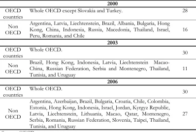
PISA was originally created by the governments of OECD countries but it has now become a major assessment tool in several countries around the world. It is an international initiative managed and oriented by the OECD carry out each three years since 2000. As we mentioned before, each Cycle of PISA has been conducted to specific cognitive areas. (2000-Reading,
[image:10.612.103.501.329.598.2]2003-Mathematics and 2006- Science).1 (See Table 1)
Table 1. Evaluated Countries in PISA.
2000
OECD countries
Whole OECD except Slovakia and Turkey. 28
Non OECD
Argentina, Latvia, Liechtenstein, Brazil, Albania, Bulgaria, Hong Kong, China, Indonesia, Russia, Macedonia, Thailand, Israel, Peru, Romania, and Chile
16
2003
OECD countries
Whole OECD.
30
Non OECD
Brazil, Hong Kong, Indonesia, Latvia, Liechtenstein Macao-China, Russian Federation, Serbia and Montenegro, Thailand, Tunisia, and Uruguay
11
2006
OECD countries
Whole OECD.
30
Non OECD
Argentina, Azerbaijan, Brazil, Bulgaria, Croatia, Chile, Colombia, Estonia, Hong Kong, Indonesia, Israel, Jordan, Kyrgyz Republic, Latvia, Liechtenstein, Lithuania, Macao, Qatar, Montenegro, Serbia, Romania, Russian Federation, Slovenia, Taipei, Thailand, Tunisia, and Uruguay
27
Source: OECD.
Adding to the cross-country comparability of PISA, the 2006 version includes an extended sample of Non-OECD countries (27), allowing the comparison between developed and less developed countries.
1
PISA assesses the competencies in mentioned areas and the test seeks to assess not merely whether students can reproduce what they have learned, but also to examine how well they can extrapolate it in understanding novel settings. PISA 2006 focused on students’
competency in science in the following aspects: Knowledge of scientific concepts;
Competencies that students need to apply in specific situations immerse in a particular scientific process; Contexts in which students encounter scientific problems and relevant
knowledge and skills are applied (e.g. making decisions in relation to personal life,
understanding world affairs); and the existence of attitudes of students towards science. (See
PISA 2006, for details). Then, PISA 2006 science questions required students to identify
scientific issues, explain phenomena scientifically and use scientific evidence. As OECD
(2007) states, “…these three competencies were selected because of their importance to the practice of science
and their connection to key cognitive abilities such as inductive/deductive reasoning, systems-based thinking,
critical decision making, transformation of information (e.g. creating tables or graphs out of raw data),
construction and communication of arguments and explanations based on data, thinking in terms of models,
and use of science” (p.36).
According to PISA, scientific literacy is associated to the ability to use scientific knowledge in order to understand and make choices about future, the natural world and other topics that affects humans. In today’s technology-based societies, there is a consensus about the importance of subjects such as science for increasing development which implies better understanding of scientific concepts and theories, and the ability to structure and solve scientific problems and they are more important and valued than ever. Given that, the relevance of measuring what are the determinants of scientific literacy and the availability of self-motivation is crucial for the future of developing countries.
questionnaires about family background, learning habits and attitudes to science, school characteristics are implemented. This is an important feature of the test because of the reported gender gaps in academic achievement due to standardized test.
3.2 Self-motivation, academic assets, and country-level effect.
In this paper, we construct a basic index of motivations towards the sciences as a proxy variable of self-motivation. The information used for the construction of this index classifies pupils into one of three levels of motivation (High, Medium, and Low) according to the answers to the following question: “How much interest do you have in learning about topics in (astronomy, human biology, and geology)?” It is important to remark that this index happens to be an instrumental measure of self-motivation, and the variable from which it is constructed, clearly is not affected by PISA’s scores, thus we avoid possible endogeneity problems. This index is complemented with the inclusion of a variable of academic assets available for each student in her or his house. The academic assets index is the sum of four dummy variables associated to the possession of academic tools such as: a desk to study, a
computer, educational software, and internet access2
. The inclusion of these assets could be subjective but they give us additional information than other traditional assets as number of books.
It is evident that OECD countries outperform in sciences the rest of the countries in the sample (See Figure 1.a). Latin American countries have a similar mean to the rest of Non-OECD countries, but with less dispersion, mainly because the latter is a more heterogeneous
group of countries (e.g. Hong Kong, Jordan, and Lithuania). A more intriguing result is
obtained from the density functions by country (Fig. 1.b), the U.S. shows a great standard deviation, even compared with that of commonly labeled as unequal countries, such as Brazil and Colombia. From this figure, the difference between the country with the lowest average performance (Kyrgyzstan) and the one with highest (Finland) is evident; both density
functions had their modes quite separately, and have almost no common area.
Finally when the relation between standard deviation and mean score by country is depicted (Fig. 1c), another unexpected finding arises, the two extreme countries, in terms of the mean score (Kyrgyzstan and Finland) have almost the same standard deviation. This finding just
2 Each asset has the same value in the index, thus the index goes from 0 to 4. Nonetheless, there is a positive
adds to the general observation that there is no clear relation between dispersion and mean score. Again the U.S. appears as one of the countries with highest standard deviation.
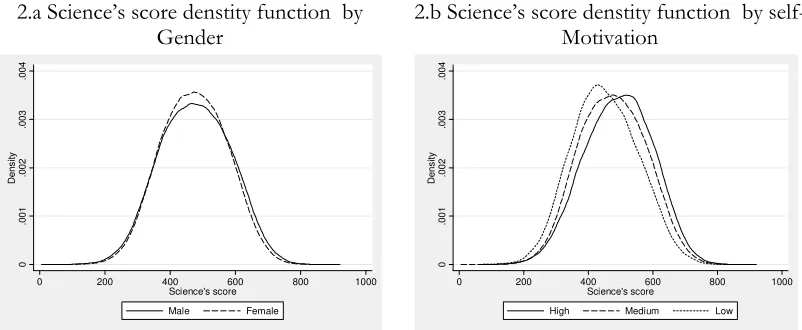
Regarding our hypothesis of the positive impact of self-motivation and academic assets at home on the student’s performance, we compute the density functions by a self-motivation and by an academic assets index.
[image:13.612.108.505.367.531.2]According to the Figure 2 both self-motivation and academic assets have a positive impact on the score’s mean. For the case of self-motivation, the change in the density function is slight, however the Kruskal-Wallis test (K-W) for equality of distribution function, rejects the equality between the score’s distributions by self-motivation level. In the case of academic assets the difference between density functions is more evident, density functions are different not only in position but also in shape; this observation is validated through the (K-W) test mentioned before.
Figure 1. Scores’ Descriptive Statistics by Region 1.a. Science’s score denstity function by
region
1.b. Science’s score denstity function by country
1.c. Science’s score (Mean Vs Standar Deviation)
Source: PISA 2006
0
.0
0
1
.0
0
2
.0
0
3
.0
0
4
De
n
s
it
y
0 200 400 600 800 1000
Science's score
Latin America OECD Others
0
.002
.0
0
4
.006
D
ens
it
y
0 200 400 600 800 Science's score
Figure 2.c. also presents the density functions by gender, in order to evaluate with our data-set the literature’s common finding of boys outperforming girls in standardized science tests. Boys have a higher mean score and a higher standard deviation which let us to say that, in terms of academic score, girls are a more homogeneous group than boys, and it also justify the necessity of using quantile regression for the comparison of this relation over different quantile of the distribution. Previous literature has been focused only in ‘average effects’ and it provides limited information about what happen in the tails of the distribution. The (K-W) test is computed, and it rejects the equality in the distribution functions of these two groups. These characteristics need to be confirmed by a conditional analysis in order to isolate the existence of confounding factors.
Figure 2.Score Density for Gender and Academic Characteristics
2.a Science’s score denstity function by Gender
2.b Science’s score denstity function by self-Motivation
2.c Science’s score density function by academic assets
Source: PISA 2006
0 .0 0 1 .0 0 2 .0 0 3 .0 0 4 De n s ity
0 200 400 600 800 1000
Science's score Male Female 0 .0 0 1 .0 0 2 .0 0 3 .0 0 4 Den s ity
0 200 400 600 800 1000
Science's score
High Medium Low
0 .0 0 2 .0 0 4 .0 0 6 Den s ity
0 200 400 600 800 1000
Science's score
3.3 Econometric exercises.
As it can be seen in the literature, most of works about the effect of changes in resources on the academic performance them do not include important aspects such as the student’s motivation. Through some econometric specifications we proof the statistical significance of the effect of self-motivation and academic assets on the pupil’s score. Whereby, we include
control variables that may be classified in three groups: i) individual features (gender, scientific
skills, and mother’s educational level); ii) school’s characteristics (private or public, and
gender); and iii) location variables (OECD membership, city’s population).
Gender, mother’s educational level, type of school (private or public), OECD membership and city’s population are included as dummy variables, where female, less than college, private, non-OECD, and village are the reference category. Science skills are measured as a principal component index, by aggregating the reported ability to understand eight different issues (health, earthquakes, antibiotics, garbage, species survival, food labels, life on Mars, and acid rain). Finally, we include a proxy variable of gender interaction within the school which is measured by the boys to total students (at the school) ratio. The purpose of this variable is to get information about the importance of coeducation or single-sex schools on the score.
Different econometric specifications were estimated in order to consider particular features
among countries that may cause systematic differences on the pupil’s performance. We also control for the differential effect of academic assets and self-motivation over the scores’ distribution. In particular, it is possible to argue that since countries have particular
educational systems (e.g. the trade-off between coverage and quality could be diverse), students
with similar profile across countries could obtain different scores. And, since self-motivation and academic assets are expected to be less disperse on the higher score’s quartiles, their impact on the results could be different along the distribution of scores.
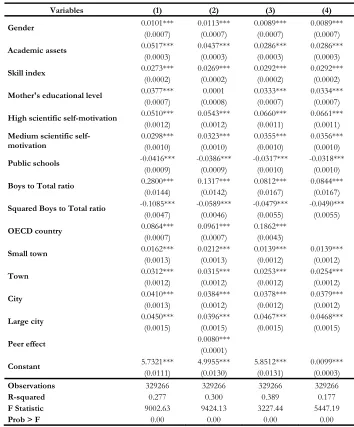
characteristics, private school’s students outperform public school’s students; and science’ score increases with the boys to total ratio. Finally, on the associated variables with our hypothesis, results support that academic assets and scientific interests are positively related with science’s scores. The former might be due to the fact that academic assets complement student’s skills and other educational inputs; and the latter, is explained by the motivation of the students to explore on specific topics, allowing her or him to deepen their understanding of scientific issues. From these findings, we can extract that there seems to have strong influences of motivation and resources on academic achievement when they are taken jointly.
Table 2. Results of Linear Regressions for Determinants of Students’ Score
Variables (1) (2) (3) (4)
Gender 0.0101*** 0.0113*** 0.0089*** 0.0089***
(0.0007) (0.0007) (0.0007) (0.0007)
Academic assets 0.0517*** 0.0437*** 0.0286*** 0.0286***
(0.0003) (0.0003) (0.0003) (0.0003)
Skill index 0.0273*** 0.0269*** 0.0292*** 0.0292***
(0.0002) (0.0002) (0.0002) (0.0002)
Mother's educational level 0.0377*** 0.0001 0.0333*** 0.0334***
(0.0007) (0.0008) (0.0007) (0.0007)
High scientific self-motivation 0.0510*** 0.0543*** 0.0660*** 0.0661***
(0.0012) (0.0012) (0.0011) (0.0011)
Medium scientific self-motivation
0.0298*** 0.0323*** 0.0355*** 0.0356*** (0.0010) (0.0010) (0.0010) (0.0010)
Public schools -0.0416*** -0.0386*** -0.0317*** -0.0318***
(0.0009) (0.0009) (0.0010) (0.0010)
Boys to Total ratio 0.2800*** 0.1317*** 0.0812*** 0.0844***
(0.0144) (0.0142) (0.0167) (0.0167)
Squared Boys to Total ratio -0.1085*** -0.0589*** -0.0479*** -0.0490***
(0.0047) (0.0046) (0.0055) (0.0055)
OECD country 0.0864*** 0.0961*** 0.1862***
(0.0007) (0.0007) (0.0043)
Small town 0.0162*** 0.0212*** 0.0139*** 0.0139***
(0.0013) (0.0013) (0.0012) (0.0012)
Town 0.0312*** 0.0315*** 0.0253*** 0.0254***
(0.0012) (0.0012) (0.0012) (0.0012)
City 0.0410*** 0.0384*** 0.0378*** 0.0379***
(0.0013) (0.0012) (0.0012) (0.0012)
Large city 0.0450*** 0.0396*** 0.0467*** 0.0468***
(0.0015) (0.0015) (0.0015) (0.0015)
Peer effect 0.0080***
(0.0001)
Constant 5.7321*** 4.9955*** 5.8512*** 0.0099***
(0.0111) (0.0130) (0.0131) (0.0003)
Observations 329266 329266 329266 329266
R-squared 0.277 0.300 0.389 0.177
F Statistic 9002.63 9424.13 3227.44 5447.19
Prob > F 0.00 0.00 0.00 0.00
Standard errors in parentheses
Though models consider different specifications, they exhibit similar results. Model (1) is the benchmark model, given that it was estimated using all control variables and applying OLS. In Model (2) mothers’ educational level average by school is included to evaluate the peer effect but, since the peer effect is strongly correlated with mothers’ educational level, the latter loses its statistical significance. Models (3) and (4), consider the same independent variables than Model (1) but, in order to approximate the idiosyncratic effects, they include country-level effect; such that, while Model (3) uses the Least Squares Dummy Variables estimator, Model (4) implements the specification in differences to the average effect, following Eq. 1 to 3,
where j represents the country-level fixed effect. Estimates from Model (4) are more
efficient than those of Model (3), because it computes the fixed effects but loses less freedom degrees.
ij ij j
ij X
Y
(1)
YijY.j
XijX.j
ij .j
(2)
ˆ
ˆ
. .j j
j
Y
X
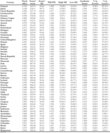
(3)The findings obtained from Models (3) and (4) support that, when they were controlled for country effect, the explanatory variables’ marginal effect is decreased, except for the
self-motivation; but in all cases, the estimated models are jointly significant. Fixed effects3
obtained from Model (4) are presented in the Table 3; measures on mean and standard deviation of the scores by country are reported, as well as self-motivation distribution and academic assets’ mean. It is easy to see that fixed effects are positively correlated with unconditional scores’ mean, where it may be highlighted that Finland and Kyrgyzstan present the highest and the lowest indicator of both fixed effect and scores’ mean. Moreover, a negative correlation between fixed effects and two estimated score’s inequality measures (quantile 90 to quantile 10
ratio) is found4
. By considering score’s dispersion measures, while Israel (score’s standard deviation and quantile 90 to quantile 10 ratio) and Kyrgyzstan (Gini) present the highest indicators, Azerbaijan shows the lowest. As a result, Azerbaijan exhibits the maximum covariance coefficient, in contrast to Kyrgyzstan.
3 By using a F test, significant differences among fixed effects were found.
4
According to our measures of academic assets and self-motivation, a positive correlation with fixed effects is found. Israel, Netherlands and Denmark reported the largest proportion of students with high scientific self-motivation (27.1%, 26%, and 24.7%, respectively), and
regarding to the academic assets index’s mean, Netherlands, Iceland, and Israel are the top
three countries (3.628, 3.596, and 3.579 respectively).
Finally, taking into account the six scientific proficiency levels5
defined from PISA scores, it is
notable that there are significant differences in the percentage of students at each level by
country. Pupils classified in higher levels have more developed scientific knowledge, and thus
are more capable to apply it in different situations. For example, according to OECD (2009) a
student in level 6 “can consistently identify, explain and apply scientific knowledge and
knowledge about science in a variety of complex life situations”, while a student at level 1
“have such a limited scientific knowledge that it can be only applied to a few, familiar
situations”. By computing the percentage of students who are at the highest level (level 6), it is
found that New Zealand, Finland and Czech Republic show the highest percentage (4.27%,
4.18% and 3.79% respectively); while some countries have no students at this level.
When this indicator is estimated for an intermediate level (level 3), there are important
changes in the order of countries. It is stressed that New Zealand remains among the
countries with the highest percentage of students at the intermediate level, while Azerbaijan
and Kyrgyzstan are the countries with the lowest values in this indicator. This implies that the
scores’ distribution by countries present significant differences, in fact, by comparing
countries’ ranking for level 6 to that of level 3 , it is obtained that the United States and Israel
are the countries with the larger negative change; in contrast to Macao and Spain, which have
the most favorable change. This ranking provides an important issue which is the differences
between OECD and non-OECD student´s representation in the upper tail of the distribution.
5 According to scores, band definition of each level is: level 1 (bellow 409.5), level 2 (409.5 to 484.1), level 3
Table 3. Fixed effects, Self-motivation, Academic Assets and scores’ level by
Country
Country Fixed effect
Scores' mean
Scores'
SD P90/P10 High SM Low SM
Academic Assets % in Level 6 % in Level 3 Finland 6.158 563.75 85.86 1.490 19.28% 18.15% 3.239 4.18% 82.31%
Japan 6.140 534.11 98.73 1.637 14.56% 24.66% 2.366 2.49% 70.51%
Czech Republic 6.099 537.72 102.85 1.677 13.59% 24.00% 3.173 3.79% 69.03%
Liechtenstein 6.097 521.86 95.93 1.638 16.22% 20.12% 3.409 2.65% 65.49%
Estonia 6.094 534.50 83.53 1.509 8.07% 29.28% 3.220 1.77% 72.58%
Chinese Taipei 6.089 543.89 91.83 1.582 9.84% 27.12% 3.146 2.10% 74.90%
New Zeland 6.087 532.31 106.93 1.715 17.63% 18.51% 3.415 4.27% 67.18%
Austria 6.078 513.84 95.36 1.648 18.51% 20.85% 3.238 1.20% 62.70%
Korea 6.076 521.69 90.55 1.581 17.62% 20.62% 3.379 1.02% 67.41%
Switzerland 6.071 507.63 95.96 1.648 19.03% 19.32% 3.365 1.13% 60.15%
Hungary 6.062 508.94 86.91 1.568 15.29% 26.96% 2.758 0.78% 61.45%
Canada 6.061 522.50 95.66 1.625 14.32% 23.06% 3.438 2.02% 65.96%
Netherlands 6.058 530.41 93.38 1.602 26.04% 10.71% 3.628 1.83% 68.77%
Germany 6.057 515.95 100.02 1.684 17.89% 21.34% 3.404 1.78% 63.83%
United Kingdom 6.049 514.34 105.94 1.736 18.11% 16.95% 3.460 2.88% 61.15%
Poland 6.047 503.02 91.23 1.623 11.69% 18.90% 2.947 0.99% 57.47%
Spain 6.047 504.45 86.54 1.567 18.19% 15.96% 3.113 0.49% 60.38%
Belgium 6.046 516.21 96.93 1.658 18.60% 22.42% 3.430 0.78% 65.02%
Ireland 6.044 509.35 94.65 1.640 22.60% 19.10% 3.188 1.18% 60.39%
Sweden 6.043 504.27 94.03 1.633 14.26% 17.52% 3.373 0.99% 58.45%
Macao 6.041 509.45 78.96 1.505 12.14% 24.50% 3.214 0.29% 62.77%
Slovak Republic 6.038 491.07 93.02 1.647 16.28% 19.33% 2.565 0.76% 52.46%
Slovenia 6.031 494.34 96.73 1.681 14.94% 30.72% 3.446 1.20% 52.87%
Denmark 6.026 495.12 92.46 1.633 24.68% 13.28% 3.437 0.77% 54.55%
Italy 6.025 487.16 96.05 1.692 10.03% 28.15% 3.083 0.62% 52.16%
Latvia 6.022 493.66 83.44 1.559 6.97% 27.69% 2.820 0.34% 54.95%
Croatia 6.019 493.31 85.10 1.573 13.05% 30.95% 2.952 0.46% 54.06%
Luxembourg 6.016 486.97 96.90 1.708 19.88% 19.50% 3.287 0.53% 52.49%
Greece 6.012 476.76 91.91 1.659 20.36% 30.58% 2.493 0.23% 49.03%
Russia 6.006 481.38 89.85 1.635 8.48% 26.76% 2.332 0.53% 48.61%
Lithuania 6.003 486.46 89.97 1.637 9.09% 30.97% 2.797 0.38% 51.50%
Iceland 5.999 490.80 96.54 1.684 14.83% 26.77% 3.596 0.61% 53.81%
Portugal 5.993 478.69 86.81 1.626 12.07% 19.05% 3.008 0.10% 48.58%
Norway 5.990 486.43 96.22 1.680 15.78% 18.77% 3.540 0.62% 51.13%
United State 5.988 488.29 105.57 1.785 13.15% 23.08% 3.279 1.64% 51.40%
Turkey 5.930 427.92 83.05 1.668 14.64% 30.19% 1.733 0.08% 23.74%
Chile 5.921 442.55 90.89 1.725 10.73% 27.36% 2.012 0.10% 31.91%
Thailand 5.920 429.99 82.76 1.642 2.27% 32.79% 1.744 0.02% 24.98%
Serbia 5.912 436.76 84.90 1.653 13.57% 33.59% 2.557 0.00% 29.37%
Israel 5.906 455.43 110.90 1.932 27.07% 22.20% 3.579 0.81% 40.40%
Uruguay 5.903 438.12 94.59 1.788 18.01% 23.87% 2.319 0.12% 31.08%
Mexico 5.894 422.46 75.62 1.596 5.30% 35.82% 1.813 0.00% 20.89%
Jordan 5.894 427.01 87.67 1.697 12.24% 24.99% 2.212 0.00% 26.18%
Indonesia 5.894 384.77 63.46 1.530 4.48% 21.63% 0.924 0.00% 6.57%
Romania 5.890 416.26 80.91 1.679 10.80% 28.72% 2.184 0.00% 20.32%
Azerbaijan 5.868 385.35 56.72 1.457 9.96% 32.18% 1.325 0.00% 5.84%
Montenegro 5.858 408.78 79.20 1.657 15.42% 38.08% 2.295 0.00% 17.46%
Tunisia 5.826 384.31 81.59 1.749 16.48% 34.03% 1.602 0.00% 12.05%
Argentina 5.825 398.91 96.63 1.907 18.79% 23.51% 1.904 0.02% 18.78%
Colombia 5.811 391.53 85.14 1.785 5.40% 43.95% 1.482 0.00% 13.62%
Brazil 5.807 385.48 90.14 1.837 14.93% 23.07% 1.720 0.03% 14.47%
Qatar 5.679 348.99 81.88 1.805 17.53% 27.49% 3.156 0.02% 6.37%
As a consequence of this fact and the fact that traditional works in the literature of economics
of education have estimated the effect of a set of variables on the ‘average’ of the population
with a non conclusive evidence, we adopt other strategy. In order to assess the effect of our
independent variables on different points of the science’s score conditional distribution, we
estimated Quantile Regression models following Kroenker and Bassett (1978). In this kind of
models, parameters are estimated minimizing the Eq. (4):
i i i i K X Y i i i i X Y i i ii X Y X
Y Min
: :
1
Where
represents the
-th quantile for which
is estimated.Mean and standard deviation of each explanatory variable by score’s quartile are summarized
in Table 4. As it can be seen, every variable exhibits important changes on both indicators
across the selected quartiles. By comparing quartile 1 with quartile 4, educative assets’ mean
increases from 2.7 to 3.37, while its standard deviation diminishes by a 40%. In the case of
self-motivation, the share of students with high and medium levels increases by 10 pp.
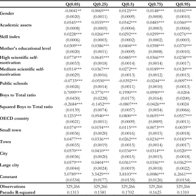
The estimated coefficients of the Quantile Regression results for 5 particular percentiles (5, 25,
50, 75 and 95) are shown in Table 5. It is worth to mention that when we compare these
results with those of OLS, the signs and significance of the coefficients do not change.
Furthermore, the goodness of fit measure indicates that our control variables have a good
explanatory power.
By examining each coefficient’s behavior along the score’s distribution6
, it is observed that the
effect of gender, public school, and boys to total ratio (squared) increase with the quantile.
The variable ‘boys to total ratio’ (lineal and squared) is not statistically significant in the highest
quartiles, while the same is observed for the gender’s effect in the lowest ones. These findings
support the pertinence of using a Quantile Regression approach when we are studying cases in
which there are considerable development differences.7
It is also important to point out that the marginal effects of OECD membership and city size
decrease. Other variables show a particular behavior; that is the case of the skills index which
has a non-monotonic shape, and mother’s educational level impact which is not statistically
[image:21.612.114.512.145.567.2]different from the OLS estimated effect.
Table 4 – Socio-economic Characteristics by score’s quartile.
Total Quartile 1 Quartile 2 Quartile 3 Quartile 4
Gender 0.495 0.499 0.479 0.480 0.521
(0.499) (0.500) (0.499) (0.499) (0.499)
Academic assets 2.780 2.002 2.604 3.074 3.374
(1.269) (1.366) (1.302) (1.079) (0.839)
Skill index 0.000 -0.705 -0.360 0.096 0.913
(1.867) (1.962) (1.801) (1.699) (1.595)
Mother's educational level 0.441 0.328 0.389 0.471 0.577
(0.496) (0.469) (0.487) (0.499) (0.494)
High scientific self-motivation
0.249 0.201 0.229 0.261 0.303 (0.432) (0.400) (0.420) (0.439) (0.459)
Medium self-motivation 0.613 0.617 0.620 0.615 0.599
(0.487) (0.486) (0.485) (0.486) (0.490)
Public school 0.820 0.885 0.840 0.793 0.759
(0.384) (0.318) (0.366) (0.404) (0.427)
Boys to Total ratio 1.501 1.516 1.501 1.494 1.495
(0.188) (0.197) (0.187) (0.184) (0.184)
Squared Boys to Total ratio
2.290 2.338 2.287 2.267 2.268 (0.576) (0.609) (0.572) (0.559) (0.561)
OECD country 0.630 0.442 0.611 0.701 0.767
(0.482) (0.496) (0.487) (0.457) (0.422)
Small town 0.225 0.257 0.231 0.213 0.197
(0.417) (0.437) (0.421) (0.409) (0.397)
Town 0.314 0.303 0.318 0.319 0.317
(0.464) (0.459) (0.465) (0.465) (0.465)
City 0.252 0.216 0.246 0.266 0.281
(0.434) (0.411) (0.430) (0.442) (0.449)
Large city 0.107 0.083 0.105 0.113 0.129
(0.309) (0.276) (0.306) (0.316) (0.335)
Source: PISA 2006. Std. Dev. in parenthesis.
For our two main interest variables (self-motivation and academic assets), their importance
decreases with the quantile but, it is always positive. This indicates that for students with the
poorest performance the tenure of academic assets and a higher level of self-motivation could
foster their academic achievements, in a more accelerated pace. This implies that a policy
oriented to elevate the pupil’s level of self-motivation towards science, would have a positive
holds for a policy directed to increase the provision of educative assets at home. Given the
expected positive relationship between information access and individual interest on a specific
topic, social programs devoted to improve the ICT’s coverage would have a positive outcome
on the student’s school performance mean and gap, through two channels: i) students with
more academic tools perform better (direct channel); ii) easier access to information has an
inertial effect, when a student meets a topic for the first time, and she or he has easy access to
more information on the subject, she or he would be motivated to deepen her or his
[image:22.612.113.515.248.651.2]knowledge on the area (indirect channel).
Table 5. Results of Quantile Regressions for Determinants of Students’ Score
Q(0.05) Q(0.25) Q(0.5) Q(0.75) Q(0.95)
Gender -0.0041** 0.0069*** 0.0125*** 0.0148*** 0.0181***
(0.0020) (0.0011) (0.0009) (0.0008) (0.0010)
Academic assets 0.0545*** 0.0559*** 0.0542*** 0.0485*** 0.0360***
(0.0008) (0.0005) (0.0004) (0.0003) (0.0004)
Skill index 0.0228*** 0.0266*** 0.0292*** 0.0299*** 0.0276***
(0.0006) (0.0003) (0.0002) (0.0002) (0.0003)
Mother's educational level 0.0309*** 0.0386*** 0.0404*** 0.0398*** 0.0370***
(0.0020) (0.0011) (0.0009) (0.0008) (0.0010)
High scientific self-motivation
0.0774*** 0.0645*** 0.0485*** 0.0366*** 0.0238*** (0.0033) (0.0018) (0.0014) (0.0014) (0.0017)
Medium scientific self-motivation
0.0514*** 0.0367*** 0.0272*** 0.0189*** 0.0120*** (0.0029) (0.0016) (0.0013) (0.0012) (0.0015)
Public schools -0.0733*** -0.0550*** -0.0392*** -0.0244*** -0.0097***
(0.0026) (0.0014) (0.0011) (0.0010) (0.0013)
Boys to Total ratio 0.7099*** 0.3776*** 0.1990*** 0.0990*** -0.0204
(0.0430) (0.0228) (0.0175) (0.0164) (0.0200)
Squared Boys to Total ratio -0.2684*** -0.1452*** -0.0807*** -0.0426*** 0.0024
(0.0139) (0.0074) (0.0057) (0.0054) (0.0066)
OECD country 0.1253*** 0.0940*** 0.0800*** 0.0695*** 0.0557***
(0.0021) (0.0011) (0.0009) (0.0009) (0.0011)
Small town 0.0374*** 0.0194*** 0.0115*** 0.0073*** 0.0039**
(0.0036) (0.0020) (0.0016) (0.0015) (0.0018)
Town 0.0477*** 0.0336*** 0.0262*** 0.0216*** 0.0183***
(0.0035) (0.0019) (0.0015) (0.0014) (0.0017)
City 0.0570*** 0.0410*** 0.0334*** 0.0314*** 0.0320***
(0.0036) (0.0020) (0.0015) (0.0015) (0.0018)
Large city 0.0579*** 0.0404*** 0.0361*** 0.0356*** 0.0362***
(0.0044) (0.0024) (0.0019) (0.0018) (0.0022)
Constant 5.0789*** 5.5429*** 5.8103*** 6.0086*** 6.2661***
(0.0334) (0.0177) (0.0135) (0.0126) (0.0154)
Observations 329,266 329,266 329,266 329,266 329,266
Pseudo R-squared 0.1313 0.1581 0.1702 0.1625 0.1310
4. Concluding Remarks
PISA 2006 allows us to have a comparable measure of school performance across developed and less developed countries and to get information on student’s self-motivation and academic assets’ tenure and its relationship with academic performance in sciences. Our findings confirm the intuition that some of the most important inputs as the self-motivation and academic tools have a positive impact on school attainment. Their effect on academic performance is different across the score’s distribution and it gives support to the importance of designing focalized programs for different populations. As a consequence of the existence of several works in which there are no consensus about the input-output relation in education, we proceed to estimate quantile regression models that, allow us to evaluate the importance of changing some inputs at different types of populations. This estimation lets us to assess whether the increase in one input (i.e. academic asset) on the student’s performance is similar over the entire population. The estimation of linear regressions with country-level fixed effects lets us to calculate the intrinsic differences between OECD and non-OECD countries, which could be used for assessing the added value of each educative system. Those countries with better socioeconomic and institutional environments need less investment to get the same performance than less developed countries.
Although, in terms of inequality we find that there is no pattern between each inequality index
and PISA score in science, the main results of the quantile regression says us that, on one
hand, the effect of gender, public school, and boys to total ratio (squared) increase with the
quantile. On the other hand, gender interaction proxied by (boys to total ratio variable) is not
statistically significant in the highest quartiles, while gender’s effect also seems to be not
significant in the lowest scores.
According to our findings, the access to modern technologies such as internet will be useful for increasing the benefits of learning when it could be used everywhere, mainly at home. Most of the great advances in education come from the creation of software packages specially designed for increasing skills such as reading comprehension, spatial analysis, and phenomena description, among others. In our case, Internet could be a substitute of another
input which is the number of books at home. The positive outcome of ICT’s on the academic
performance mean and gap, may occur through two channels: i) students with more academic
tools perform better (direct channel); ii) easier access to information has an inertial effect on
students’ proclivity to deepen their knowledge (indirect channel). However, it is important to
technology gap between students because those without access will be in less favorable
conditions with respect to those who have access in their households.
Therefore, public policy in education in less developed countries has to increase investments in modern pedagogy techniques in order to increase motivation levels and it should take into
account differences in initial endowments of populations. Finally, it seems to be a strong link
between academic assets and self-motivation, which is an important result if we consider that in some cases parents could invest in materials but they do not success in translate their preferences into student’s motivations.
References
Al Samarrai, S., 2002. Achieving Education for All: How Much Does Money Matter?. Journal of International Development 18 (2), 179 – 206.
Altinok, N., Bennaghmouch, S., 2008. School Resources and the Quality of Education: Is there a link. Association Francaise de Cliometrie. Working Papers, No.1
Altinok, N., 2007. A Macroeconomic Estimation of the Education Production Function. IREDU-Working Paper.
Benbow, C., Stanley, J., 1980. Sex Differences in Mathematical Ability: Fact or Artifact?. Science 210 (4475), 1262 – 1264.
Betts, J., 1996. The Role of Homework in Improving School Quality. Discussion Paper 96-16. Department of Economics, UCSD.
Betts, J., 1998. The Impact of Educational Standards on the Level and Distribution of Earnings. American Economic Review 88 (1), 266–275.
Bishop J., Woessmann, L., 2004. Institutional Effects in a Simple Model of Educational Production. Education Economics 12 (1), 17-38.
Bishop, J., 1989. Is the Test Decline Responsible for the Productivity Growth Decline?. American Economic Review 79(1), 178-197.
Bishop, J., 1992. The Impact of Academic Competencies on Wages, Unemployment, and Job Performance, Carnegie-Rochester Conference. Series on Public Policy 37, 127-194. Bishop, J., 1997. The Effect of National Standards and Curriculum - Based Exams on
Achievement. American Economic Review, Papers and Proceedings87(2), 260-264.
Bishop, J., 1999. Are National Exit Examinations Important for Educational Efficiency?.
Swedish Economic Policy Review6(2), 349-398.
Bishop, J., 2006. Drinking from the Fountain of Knowledge: Student Incentive to Study and Learn Externalities, Information Problems and Peer Pressure. In: Handbook of the Economics of Education, Vol 2. Ed Eric Hanushek and Finis Welch. Elsevier.
Bishop, J., Bishop, M., Gelbwasser, L., Green, S., Zuckerman, A., 2003. Nerds and Freaks: A Theory of Student Culture and Norms. In: Ravitch, D. (Ed.), Brookings Papers on Education Policy. Brookings Institution Press, Washington, DC, 141–213.
Boissiere M., Knight, J.B., Sabot, R.H., 1985. Earnings, Schooling, Ability, and Cognitive Skills. American Economic Review 75(3), 1016-1030.
Checchi, D., Peragine, V., 2005. Regional Disparities and Inequality of Opportunity: The Case
Chen, Z., West, E., 2000. Selective versus Universal Vouchers: Modelling Median Voter Preferences in Education. American Economic Review 90(5), 1520-1534.
Chiu M.M., Xihua, Z., 2008. Family and Motivation Effects on Mathematics Achievement: Analyses of Students in 41 Countries. Learning and Instruction 18, 321-336.
Colclough C., Lewin, K., 1993. Educating All the Children: Strategies for Primary Schooling in the South, Clarendon Press, Oxford.
Coleman, J.S., Campbell, E.Q., Hobson, C.J., Mcpartlet, J., Mood, A., Weinfeld, F.D., York, R.L., 1966. Equality of Educational Opportunity, Washington, D.C. U.S. Government Printing Office.
Cooper, H.M., 1989. Homework. Longman, White Plains, New York.
Costrell, R., 1994. A Simple Model of Educational Standards. American Economic Review 84(4), 956–971.
Datar A., Mason, B., 2008. Do Reductions in Class Size “Crowd Out” Parental Investment in Education?. Economics of Education Review 27, 712-723.
Deci, E.L., Vellerand, R., Pelletier, L., Ryan, R., 1991. Motivation and Education. Educational Psychologist 26 (34), 324-346.
Dzama E., Osborne, J.F., 1999. Poor Performance in Science among African Students: An Alternative Explanation to the African Worldview Thesis. Journal of Research in Science Teaching 36(3), 387–405.
Eide E., Showalter, M., 1998. The Effect of School Quality on Student Performance: A Quantile Regression Approach. Economic Letters 58, 345-350.
Epple, D., Romano, R., 1998. Competition between Private and Public Schools, Vouchers, and Peer-Group Effects. American Economic Review 88(1), 33-62.
Fuchs, T., Woessmann, L., 2008. What Accounts for International Differences in Student Performance? A Re-examination using PISA Data. In: Physica-Velrlag HD., (Ed.), The Economics and Training of Education, 209-240.
Gottfried A.E., Fleming, J., Gottfried, A.W., 1998. Role of Cognitively Stimulaton Home Environment in Children’s Academic Intrinsic Motivation: A Longitudinal Study. Child Development 69 (5), 1448-1460.
Gupta S., Verhoeven, M., Tiongson, E., 2002. The Effectiveness of Government Spending on Education and Health Care in Developing and Transition Countries. European Journal of Political Economy 18, 717-737.
Hanushek, E.A., 1986. The economics of Schooling: Production and Efficiency in Public Schools. Journal of Economic Literature XXIV, 1141-1177.
Hanushek, E.A., 1998. Conclussion and Controversies about the Effectiveness of School Resources. Economic Policy Review, Federal Reserve Bank of New York 4(1), 11-28. Hanushek, E.A., Kimko, D.D., 2000. Schooling, Labor - force Quality and the Growth of
Nations. American Economic Review 22(5), 1184-1208.
Hanushek, E.A., 1994. Making Schools Work: Improving Performance and Controlling Costs. Brookings Institution Press, Washington, DC.
Houtenville, A.J., Smith, K., 2008. Parental Effort, School Resources, and Student Achievement. Journal of Human Resources 43(2), 437-453.
Hoxby, C., 2000. The effects of class size on student achievement: New evidence from population variation. Quaterly Journal of Economics 115(4), 1239-1285.
Hoxby, C., 1999. The Productivity of Schools and Other Local Public Goods Producers. Journal of Public Economics 74(1), 1-30.
Hyde, J., Fennema, E., Lamon, S., 1990. Gender Differences in Mathematics Performance: A
Meta-analysis. Psychology Bulletin 107(2), 139-155.
Krueger, A., 1998. Reassesing the View that American Schools are Broken. Economic Policy
Review, Federal Reserve Bank of New York 4(1), 29-46.
Lee, J.W., Barro, R.J., 2001. Schooling Quality in a Cross Section of Countries. Economica 38 (272), 465-488.
Mcmahon W., 1999. Education and Development: Measuring the Social Benefits, Oxford University Press, Oxford.
Meece, J., Glienke, B.B., Burg, S., 2006. Gender and Motivation. Journal of School Psychology 44, 351-373.
Moll, P.G., 1998. Primary Schooling, Cognitive Skills, and Wage in South Africa. Economica 65, 263–284.
Nechyba, T., 1999. School Finance Induced Migration and Stratification Patterns: The Impact
of Private School Vouchers.Journal of Public Economic Theory 1(1), 5-50.
Nechyba, T., 2000. Mobility, Targeting, and Private-School Vouchers. American Economic Review 90(1), 130-146.
Nechyba, T., 2003. School Finance, Spatial Income Segregation, and the Nature of Communities. Journal of Urban Economics 54(1), 61-88.
OECD, 1999. Measuring Student Knowledge and Skills: A New Framework for Assessment. Retrieved September 2009 from www.pisa.oecd.org.
OECD, 2007. PISA 2006 Science Competencies from Tomorrow´s World, vol. 1. Analysis. Retrieved October 2009 from www.pisa.oecd.org.
OECD, 2009. PISA 2006. Technical Report. Retrieved October 2009 from www.pisa.oecd.org.
Peragine, V., Serlenga, L., 2007. Higher Education and Equality of Opportunity in Italy. IZA Discussion paper series, DP No. 3163.
Psalidas, A., Apostolopoulos, C., Hatzinikita, V., 2008. Investigating Factors Affecting Students’ Performance to PISA Science Items. Journal of Engineering Science and Technology Review 1, 90-97.
Schultz, T.P., 1995. Accounting for Public Expenditures on Education: An International Panel Study. In:Schultz, T.P., (ed.), Research in Population Economics 8, Greenwich, CT, JAI Press.
Stinebrickner, T., Stinebrickner, R., 2007. The Causal effect of Studying on Academic Performance. NBER Working paper series 13341.
Sula, O., 2008. Demand for International Reserves: A Quantile Regression Approach. MPRA,
Paper No 11680.
Walter J., Hart, J., 2009. Understanding the Complexities of Student Motivations in Mathematics Learning. Journal of Mathematical Behavior 28, 162-170.
Woessmann, L., 2003. Schooling Resources, Educational Institutions, and Student Performance: The International Evidence. Oxford Bulletin of Economics and Statistics 65(2), 117-170.
28