Topological Behavior of Families of Algebraic Curves Continuously Depending on a Parameter Under Certain Conditions
14
0
0
Texto completo
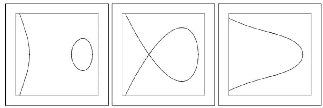
(2) Mathematics Classification: 68W30, 14Q99.. 1. Introduction. In previous works ((1), (2)) we addressed the following problem: given a family of algebraic curves algebraically depending on a parameter t ∈ R, therefore represented by a real polynomial f (x, y, t), compute the different shapes arising in the family, and the t-values corresponding to each shape. In (2) an algorithm for solving this question was provided (the same algorithm was adapted in (3) to the case when the family was rational, in order to work directly in parametric form, therefore in a more efficient way). By using the algorithm in (2), one can compute, for example, the different shapes arising in the family f (x, y, t) = t(x + y 2 − 1) + (t − 1)2 (x3 + y 2 − x2 ) = 0 More precisely, in this case one has three topology types, shown in Figure 1, corresponding to t ∈ (−∞, 0) (see Fig. 1, left), t = 0 (see Fig. 1, center) and t ∈ (0, ∞) (see Fig. 1, right), respectively.. Fig. 1. Shapes in the family t(x + y 2 − 1) + (t − 1)2 (x3 + y 2 − x2 ) = 0. The algorithm in (2) is of interest in contexts where geometrical objects depending on parameters may appear, for example in the topological analysis of the solutions of first-order differential equations, in robotics, in Computer Aided Geometric Design, in Control Theory, in Algebraic Biology, etc. Also of interest in these contexts, in this paper we consider the same problem but for a wider class of families of algebraic curves, also depending on a real parameter but where the dependence of the parameter is continuous, but not necessarily algebraic. So, we consider the problem of computing the shapes arising in families like, for instance, f (x, y, t) = y 4 + log(t2 + 1)xy 2 − |t|y + t2 + 1 = 0, with t ∈ R. The topology types arising in this family are computed in Example 2, Section 4 of this paper. In order to solve this question, based on (2) and 2.
(3) on classical results on the specialization of resultants, we first develop some results on families of algebraic curves algebraically depending on finitely many parameters. Then, exploiting these results and using properties of continuous functions, we provide, for a given family of the considered type, a method for computing a real function R(t⋆ ) with the following property: whenever R(t⋆ ) is not identically 0, the topology type of the family is invariant along every real interval I ⊂ R where f is defined, not containing any real root of R(t⋆ ); thus, the topology of the family along I can be described by taking a representative t0 ∈ I, and computing the topology of the curve described by f (x, y, t0 ) (see (5),(6),(8)). An important case where R(t⋆ ) can be guaranteed to be different from 0 happens when all the coefficients f (x, y, t) are algebraically independent, or can be expressed in terms of algebraically independent functions (see Corollary 11). Hence, under that condition the method is always successful. When R(t⋆ ) is identically 0, the method fails. At the moment we are unaware of a solution for this special case, that we pose here as an open problem. Nevertheless, at the end of the paper (see Section 5) we make some observations on this special case, and we connect it with a topological problem. The structure of the paper is the following. In Section 2 we briefly recall some ideas and results of (2) that are needed for developing the results of the paper. In Section 3, some results on families of algebraic curves depending on finitely many parameters are provided. In Section 4, these results are used to provide the main result of the paper. Some general considerations on the special case R(t⋆ ) = 0 are made in the last section of the paper.. 2. Previous Results. Let F = F (x, y, t) be a real polynomial in the variables x, y, t. Given t0 ∈ R such that F (x, y, t0) = Ft0 (x, y) is not identically 0, Ft0 (x, y) defines a plane algebraic curve Ct0 . Hence, we can consider F as defining a family of algebraic curves F algebraically depending on the parameter t. Clearly, as t0 moves in R the shape of Ct0 may change. So, it has sense to address the problem of detecting the different topology types arising in F . Moreover, by Hardt’s Semialgebraic Triviality Theorem (see Theorem 5.46 in (4)), the number of different topology types in the family must be necessarily finite. In order to solve this problem, the following definition is introduced: Definition 1 Let A ⊂ R. We say that A is a critical set of the family defined by F , if for all ti , ti+1 ∈ R satisfying that [ti , ti+1 ] ∩ A = ∅, the topology types of Fti and Fti+1 are equal. 3.
(4) Hence, a critical set is essentially a real set containing all the values of the parameter where the topology of the family may change. In (2) an almost identical definition is provided; the difference between the definition in (2) and the above one is that in (2) a critical set is defined as a finite real set satisfying the condition in Definition 1, and the definition here does not require the set to be finite. Notice that if a finite critical set A = {a1 , . . . , ar } is computed, then the different topology types in the family can be derived. Indeed, in that case the parameter space (R, in this case) can be decomposed as (−∞, a1 ) ∪ {a1 } ∪ (a1 , a2 ) ∪ · · · ∪ {ar } ∪ (ar , +∞) Then, taking a representative for each element of the above partition, and applying standard methods ((5), (6), (8)) for describing the topology of an algebraic curve, the topology types in the family can be computed. So, in order to determine the topology of the family, the crucial question is the computation of a finite critical set. This is exactly the problem addressed in (2). Hence, we recall now the main ideas in (2). In (2) the following hypotheses on F (that we denote as (I) and (II)) are required: (I) F is square-free (as a polynomial in the variables x, y); (II) lcoeff y (F ) does not depend on the variable x. Notice that (II) can always be achieved by applying if necessary a change of coordinates of the type x = aX + bY, y = cX + dY , which does not change the topology of the family; furthermore, (II) holds trivially if degy (F ) = 0. In (2), it is also required, as a first hypothesis, the non-existence of t0 ∈ R so that Ft0 (x, y) is identically 0. This hypothesis is formulated in order to ensure that every specialization of the parameter t defines a curve of the family; however, the results in (2) can be perfectly developed excluding this hypothesis. Thus, in the present work we will not take it into account. Furthermore, we need to introduce two polynomials; here, Dw (G) := Resw (G, ∂G ), ∂w √ and G denotes the square-free part of G. Also, abusing of language, in the sequel we will refer to Dw (G) as the “discriminant” of G w.r.t. the variable w (notice that usually the discriminant denotes the result of dividing out the resultant Dw (G) by the leading coefficient). Then we define (this notation is slightly different to that of (2), and was suggested by an anonymous postreviewer of the paper (2)),. M(x, t) :=. R(t) :=. q Dy (F (x, y, t)) F (x, t) Dx (M(x, t)) . M(t). 4. if degy (F ) 6= 0 if degy (F ) = 0. if degx (M) 6= 0 if degx (M) = 0. ,.
(5) With this definition, the following lemma holds. Lemma 2 The polynomial R(t) is identically 0 iff F (x, y, t) is identically 0. Proof. By the definition of M, it holds that M is either square-free, or constant. Indeed, this is clear if degy (F ) 6= 0; if degy (F ) = 0, M is defined as F , and since by hypothesis F is square-free, then so is M. Hence, let us see (⇒). If R = 0 then M = M(t), because otherwise we would have that Dx (M) = 0 and therefore M would not be square-free. But then by definition of R we have R = M, and therefore M = 0. Now by the definition of M, and taking again into account that F is square-free by hypothesis, we conclude that F = 0. (⇐) is straightforward from the definitions of M, R. Thus, the following theorem, which provides a method for computing a finite critical set, holds (see Theorem 4 and Theorem 13 in (2)). Theorem 3 Let F satisfy the hypotheses (I) and (II). Then the set of real roots of R, is a critical set of F . If R has no real roots, then the elements of the family show just one topology type.. 3. Families of Algebraic Curves Algebraically depending on parameters. In Section 2 we have revised known results concerning families of algebraic curves algebraically depending on a parameter. Based on these ideas, in this section we provide some results for families of algebraic curves algebraically depending on finitely many parameters. So, let F ∈ R[x, y, t1 , . . . , tn ] be a real polynomial in the variables x, y, t1, . . . , tn satisfying the conditions (I), (II) introduced in Section 2, where t1 , . . . , tn are parameters taking values in R; in other words, F is square-free as a polynomial in the variables x, y and lcoeff y (F ) does not depend on x. Hence, for each specification of (t1 , . . . , tn ) = (a1 , . . . , an ) ∈ Rn in F (except for those ones causing F to be identically 0), the polynomial Fa1 ,...,an (x, y) obtained this way defines an algebraic curve. In particular, one may consider F as defining a family F of algebraic curves algebraically depending on the parameters t1 , . . . , tn . Also from Hardt’s Semialgebraic Triviality Theorem, it follows that the number of these types must be finite. So, our purpose is to apply the results in the above section in order to study the topology types in F . The definitions of the polynomials M, R provided in Section 2 are easily gen5.
(6) eralized for the case of several parameters. Hence, we define q Dy (F (x, y, t1 , . . . , tn )). M(x, t1 , . . . , tn ) :=. R(t1 , . . . , tn ) :=. F (x, t1 , . . . , tn ) Dx (M(x, t1 , . . . , tn )) . M(t1 , . . . , tn ). if degy (F ) 6= 0. ,. if degy (F ) = 0. if degx (M) 6= 0 if degx (M) = 0. Notice that degy (F ) 6= 0 (resp. degx (M) 6= 0) iff lcoeff y (F ) (resp. lcoeff x (M)) is not identically 0. Furthermore, reasoning as in Lemma 2, we have the following result. Lemma 4 The polynomial R(t1 , . . . , tn ) is identically 0 iff F (x, y, t1 , . . . , tn ) = 0. Now, in the sequel, if G is a polynomial depending on the parameters t1 , . . . , tn (maybe depending also on other variables), we denote the evaluation of G at t1 = a1 , . . . , tn = an as Ga1 ,...,an . So, Fa1 ,...,an , Ma1 ,...,an , Ra1 ,...,an denote the evaluations of F, M, R at t1 = a1 , . . . , tn = an , respectively. Notice that Fa1 ,...,an = Fa1 ,...,an (x, y), and Ma1 ,...,an = Ma1 ,...,an (x). Thus, a first problem is to decide whether M and R behave well under the specialization of the parameters t1 , . . . , tn . In order to make this idea more precise, we introduce the following additional notation; for (a1 , . . . , an ) ∈ Rn , we define M̃ (x, a1 , . . . , an ) :=. R̃(a1 , . . . , an ) :=. q Dy (Fa. 1 ,...,an. (x, y)) if degy (Fa1 ,...,an ) 6= 0. Fa1 ,...,an (x) Dx (Ma ,...,a (x)) n. if degx (Ma1 ,...,an ) 6= 0. Ma1 ,...,an. if degx (Ma1 ,...,an ) = 0. 1. . ,. if degy (Fa1 ,...,an ) = 0. Notice that the above polynomials are really the specializations of M, R at t1 = a1 , . . . , tn = an , since there we are taking into account how the degrees of F, M w.r.t y, x, respectively, specialize at t1 = a1 , . . . , tn = an (however, when we substitute t1 = a1 , . . . , tn = an in M, R to get Ma1 ,...,an , Ra1 ,...,an we are not considering this). Then the question is to check whether the equalities M̃ (x, a1 , . . . , an ) = Ma1 ,...,an (x), R̃(a1 , . . . , an ) = Ra1 ,...,an hold or not, i.e. whether M and R behave well under specialization, or not. A simple example will show that these polynomials do not necessarily specialize well; for example, taking F (x, y, a) = ay 2 + y + x + 1 one may see that M(x, a) = 4xa2 + 4a2 − a, R(a) = 4a2 , and therefore that M0 (x) = M(x, 0) = 0, R0 = R(0) = 0. However, F (x, y, 0) = y + x + 1, and therefore M̃0 (x) = M̃(x, 0) = 1, R̃0 = R̃(0) = 1 (from the definition of R̃). 6.
(7) First, we need the following lemma. Lemma 5 Let (a1 , . . . , an ) ∈ Rn so that Ra1 ,...,an 6= 0. Then, the following statements are true: (i) degy (Fa1 ,...,an ) = degy (F ) (ii) Fa1 ,...,an (x, y) is either non-depending on x, y, or square-free as a polynomial in x, y. Proof. Let us see (i). If degy (F ) = 0 then the statement is obvious, so assume that degy (F ) > 0. Then, let A := lcoeff y (F ). By using the Sylvester form of the resultant, one deduces that A divides M. If degx (M) = 0 then by the definition of R it also holds that A divides R; otherwise, denoting B := lcoeff x (M), also by the Sylvester form of the resultant one deduces that B divides R, and since A divides B, A divides R. Then, A(a1 , . . . , an ) 6= 0 because otherwise Ra1 ,...,an = 0, which cannot happen by hypothesis. Hence, (i) holds. Now let us see (ii), and for this purpose we distinguish the cases degy (F ) = 0 and degy (F ) 6= 0. We start with degy (F ) = 0; in this case, by the definition of M we have M = F . If degx (F ) = 0 then F is non-depending on x, y, and (ii) holds. Otherwise, degx (F ) 6= 0 and by the definition of R we have R = Dx (F ). As we have seen, B = lcoeff x (F ) is a factor of R. Hence, lcoeff x (F ) cannot vanish at (a1 , . . . , an ) because Ra1 ,...,an 6= 0 by hypothesis. Then, by Lemma 4.3.1, pg. 96 in (10) it follows that the resultant Resx (F, Fx ) specializes well, and this resultant is exactly Dx (M). Hence, if Fa1 ,...,an (x, y) is not square-free, we get that Dx (M) vanishes at (a1 , . . . , an ), which is in contradiction withqthe fact that Ra1 ,...,an 6= 0. Now, consider the case degy (F ) 6= 0. Here, M = Dy (F ). Now since statement (i) holds, we have that lcoeff y (F ) does not vanish at (a1 , . . . , an ) and therefore also by Lemma 4.3.1, pg. 96 in (10), the resultant Resy (F, Fy ) specializes well; however this resultant is Dy (F ). Since, reasoning as before, the resultant Resx (M, Mx ) also specializes well in the considered case, we get that if Fa1 ,...,an (x, y) is not square-free, then Ra1 ,...,an = 0, which cannot happen. Now we can prove the following result on the specialization of M, R. In order to prove it, one would use Lemma 5, and similar considerations to those in the proof of Lemma 5; hence, it is left to the reader. Lemma 6 Let (a1 , . . . , an ) ∈ Rn so that Ra1 ,...,an 6= 0. Then, the following statements hold: (i) M̃(x, a1 , . . . , an ) = Ma1 ,...,an (x). (ii) R̃(a1 , . . . , an ) = Ra1 ,...,an . A consequence of Lemma 5 and Lemma 6 is the following result, which is essential for our purposes. This proposition ensures that under certain condi7.
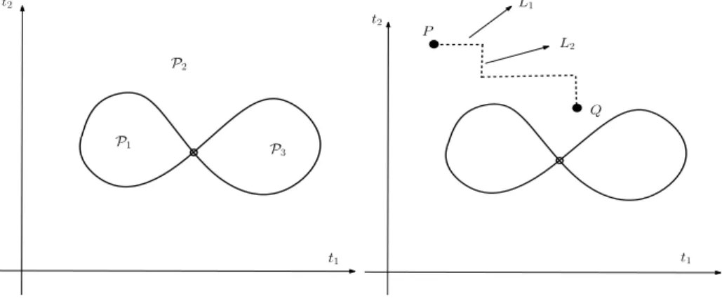
(8) tions, when we specialize all the parameters ti ’s except but one a critical set of the uniparametric family can be determined by computing the real roots of the specialization of R. For simplicity, in the statement of the result we assume that the only parameter that we do not specialize is t1 ; clearly, the statements holds if we consider any other ti , with i = 2, . . . , n. Proposition 7 Let (a2 , . . . , an ) ∈ Rn−1 , where R(t1 , a2 , . . . , an ) is not identically 0, and let G(x, y, t1 ) = F (x, y, t1 , a2 , . . . , an ). Then, the set of real roots of R(t1 , a2 , . . . , an ) is a critical set of the family defined by G. Proof. By statement (ii) of Lemma 5 it holds that G is square-free as a polynomial in x, y. Moreover, because of statement (i) of Lemma 5 we have that degy (G) = degy (F ). In particular, lcoeff y (G) is the evaluation of lcoeff y (F ) at t2 = a2 , . . . , tn = an , and this evaluation is not identically 0. Since by hypothesis lcoeff y (F ) does not depend on x, then lcoeff y (G) does not depend on x, either. Therefore, G satisfies the hypotheses (I) and (II); so, by Theorem 3, the set of real roots of R̃(t1 , a2 , . . . , an ) is a critical set of the family defined by G. However, for all t1 ∈ R so that R(t1 , a2 , . . . , an ) 6= 0, by Lemma 6 we have that R̃(t1 , a2 , . . . , an ) = R(t1 , a2 , . . . , an ). Thus, the only t1 -values where R̃(t1 , a2 , . . . , an ) can vanish are the real roots of R(t1 , a2 , . . . , an ), and hence the proposition follows. Then we are finally ready to prove the main result of this subsection. For this purpose, we denote the variety defined in Rn by R(t1 , . . . , tn ) = 0 as R. Since by Lemma 4 the polynomial R is not identically 0, then R is a proper variety, and divides Rn into open connected regions P1 , . . . , Pℓ (see Figure 1, left). Then, the following theorem, whose proof is illustrated in Figure 2, right, holds. Theorem 8 The topology type of F is invariant along each Pi . Proof. Let i ∈ {1, . . . , ℓ}, and let us prove that the topology type of F is constant over Pi . Since Pi is connected, given two points P, Q ∈ Pi we can connect them by means of finitely many oriented segments L1 , . . . , Lr satisfying the following conditions: (i) the start point of L1 is P , and the end point of Lr is Q; (ii) the end point of Lj , is the start point of Lj+1 ; (iii) along each segment Lj , all the parameters but one are constant (i.e. each segment is parallel to some coordinate axis of Rn ). Now let Lu be one of these segments, and w.l.o.g. assume that t1 is the only parameter which is not constant over Lu , i.e. the points of Lu satisfy t2 = a2 , . . . , tn = an with (a2 , . . . , an ) ∈ Rn−1 . Then, over Lu we have that G = F |Lu defines a uniparametric family of algebraic curves of parameter t1 . Now by Proposition 7, the set of real roots of R(t1 , a2 , . . . , an ) form a critical set of G. Finally, since Lu lies in Pi , then R does not vanish along Lu , and neither does R(t1 , a2 , . . . , an ). Therefore, by Theorem 3 the topology type of G, and therefore of F , stays invariant along 8.
(9) Lu . Since this holds for u ∈ {1, . . . , r}, we conclude that the topology type of F at P and Q is the same. Finally, P and Q are generic, and therefore the statement holds. t2. L1 t2. P. L2. P2 Q. P1. P3. t1. t1. Fig. 2. Theorem 8: notation (left) and proof (right).. 4. Families of Algebraic Curves Continuously depending on a parameter.. Let U[t] be the ring of continuous functions in the variable t, over a subset U ⊂ R; for simplicity we will assume that U is a real open interval, though the results are easily generalized for the case when U is the union of finitely many real intervals. Now let us consider the ring U[t][x, y]; the elements of U[t][x, y] are polynomials in the variables x, y with coefficients in U[t], i.e. f (x, y, t) =. m X n X. aij (t)xi y j. i=0 j=0. where the aij (t)’s are continuous. Given f ∈ U[t][x, y], for every t0 ∈ R so that f (x, y, t0) = ft0 (x, y) does not identically vanish one has that ft0 (x, y) defines an algebraic curve. So, one may consider that f ∈ U[t][x, y] defines a family FU of algebraic curves depending on the parameter t, with t ∈ U ⊂ R. We say that such a family is a family of algebraic curves continuously depending on the parameter t. Once again, by Semialgebraic Hardt’s Triviality Theorem such a family contains finitely many topology types. So, here we address the algorithmic analysis of these topology types. Moreover, in the sequel we will also assume that lcoeff y (f ) does not depend on x (otherwise, as observed in Section 2, one can apply an affine change of coordinates involving just x, y, which therefore does not change the topology of the family). Now let us consider the following definition, which is a generalization of Definition 1 to this new context. 9.
(10) Definition 9 Let U ⊂ R in the above conditions. Then, we say that A ⊂ R is a critical set of the family FU , if A contains all the t-values where the topology type of FU over U changes. Therefore, our aim is to compute a critical set of FU ; for this purpose, we will make use of the ideas in Section 3. We need to introduce some notation. Let f ∈ U[t][x, y], having N different terms, that we will denote as b1 (t), . . . , bN (t). Moreover, whenever bi (t) is non-constant, let us denote by F the result of performing the substitution bi (t) := ui (where ui is a new variable) in f , for i = 1, . . . , N. Notice that F is a polynomial in the variables x, y, u1, . . . , uN ; one may also see F as defining a family of algebraic curves depending on the parameters u1 , . . . , uN . Moreover, we assume that F is squarefree as a polynomial in x, y (if it is not, we compute its square-free part and we carry on the analysis; notice that substituting back ui := bi (t), the resulting polynomial defines the same family than f ). Hence, starting from F one can compute the polynomials M(x, u1 , . . . , uN ) and R(u1 , . . . , uN ) introduced in Section 3. We will write Rf (u1 , . . . , uN ) instead of simply R(u1 , . . . , uN ), to emphasize that this polynomial has been obtained from f . Moreover, let R⋆ (t) := Rf (b1 (t), . . . , bN (t)), i.e. the result of performing the “inverse substitution” ui := bi (t) in Rf for all i ∈ {1, . . . , N}. Then the following theorem, which is the main result of the paper, holds. Theorem 10 Let I ⊂ U be a real interval so that R⋆ (t) does not vanish over I. Then, the topology type of FU stays invariant along I. Proof. Since Rf is a polynomial and the bi (t)’s are continuous over I, it follows that R⋆ (t) is also continuous over I. Also, since by Lemma 4 it holds that Rf (u1, . . . , uN ) is not identically 0, then it defines a proper algebraic variety over RN that we represent by VR (if Rf is constant, VR = ∅). Now, I is connected and R⋆ (t) is continuous; therefore, R⋆ (I) is a connected subset of RN . Moreover, since R⋆ (t) does not vanish over I, this means that for t ∈ I, the curve L of RN parametrized as x1 = b1 (t), . . . , xn = bn (t) does not intersect VR when t ∈ I; indeed, if P ∈ L ∩ VR , then P = (b1 (t⋆ ), . . . , bN (t⋆ )) where R⋆ (t⋆ ) = 0. And since R⋆ (I) is connected, we deduce that for t ∈ I, L is contained in one of the connected components of RN \VR . Then the statement follows from Theorem 8. In other words, whenever R⋆ (t) is not identically 0 we have that the set A of real roots of R⋆ (t) over U is a critical set of FU . Theorem 10 provides the following corollary. Here, the notion of algebraic dependence is used. Essentially, we say that several functions α1 (t), . . . , αr (t) are algebraically dependent, if there exists a polynomial G(x1 , . . . , xr ) such that G(α1 (t), . . . , αr (t)) = 0; in other words, if there exists an algebraic relationship among them. For example, α1 (t) = sin(t) and α2 (t) = cos(t) are algebraically dependent, and G(x1 , x2 ) = x21 + x22 − 1 provides an an algebraic relationship involving them. 10.
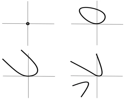
(11) We say that α1 (t), . . . , αr (t) are algebraically independent, if they are not algebraically dependent. The problem of detecting whether a given set of explicit functions is algebraically independent or not has been considered, and is still open. The reader may find some results on this question in (7); in that paper, one may find several examples of families of real functions which are algebraically independent. So, the following corollary holds. Corollary 11 If the ai,j (t)’s are algebraically independent, then the method provided for computing a critical set, is successful. Proof. If R⋆ (t) is identically 0, then R(b1 (t), . . . , bn (t)) = 0 provides an algebraic relationship satisfied by b1 (t), . . . , bn (t). So, an algebraic relationship among the ai,j (t)’s exists. However, if the ai,j (t)’s are algebraically independent, this cannot happen. The following observations should also be taken into account: (i) Unlike it happens in the case when the dependence of t is algebraic, i.e. when f ∈ R[x, y, t], it may happen that R⋆ (t) has infinitely many real roots. (ii) If R⋆ (t) has r real roots in U, then there are at most 2r + 1 topology types of FU over I. Moreover, in order to determine them one computes the real roots of R⋆ (t), and proceeds as suggested in Section 2. (iii) The set of exp-log functions (see (9) for further information) is the smallest set of functions R → R containing exp, log, the identity function and the constant functions, closed under addition, multiplication and composition of functions. It is known that every exp-log function has finitely many real roots. Hence, if the coefficients of f are independent exp-log functions, then R⋆ (t) is a non-identically 0 exp-log function as well, and the critical set determined by applying Theorem 10 is finite. Moreover, in this case there are efficient algorithms to compute the real roots of R⋆ (t) (see (9)). The following examples illustrate Theorem 10. Example 1 Consider the family F of algebraic curves defined by √ f (x, y, t) = y 4 + et xy 2 − ty + x2 Observe that the coefficients of f are continuous for t ∈ U = (0, ∞). Hence, t let us compute √ the topology types of FU . For this purpose, we consider u1 := e and u2 := t, and F (x, y, u1, u2 ) := y 4 + u1 xy 2 − u2 y + x2 Hence, we get M = −4u31 u22 x3 − 27u42 + 16u41 x6 − 128u21 x6 + 144u1x3 u22 + 256x6 , and R = −8916100448256u220(u1 − 2)6 (u1 + 2)6 (12 + u21 )9 . So, R⋆ (t) = −8916100448256 · t10 (et − 2)6 (et + 2)6 (e2t + 12)9 11.
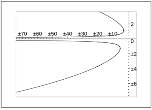
(12) which has just one real root in U, namely log 2 (here, log denotes the natural logarithm). Hence, from Theorem 10 it holds that A = {log 2} is a critical set. Then, we get at most 4 topology types, corresponding to the following cases: (I) t = 0; (II) t ∈ (0, log 2); (III) t = log 2; (IV) t ∈ (log 2, ∞). These topology types are shown in Figure 3 (the pictures here have been obtained with Maple’s package algcurves).. Fig. 3. Topology Types in Example 1: (I) up, left; (II) up, right; (III) down, left; (IV) down, right. Example 2 Let F be the family defined by f (x, y, t) = y 4 + log(t2 + 1)xy 2 − |t|y + t2 + 1 The coefficients of f are continuous for t ∈ R. In this case, we get that R⋆ (t) = −4096 log(t2 + 1)16 (t2 + 1)|t|4 (4096(t2 + 1)3 + 27|t|4 )3 The only real root of R is 0; hence, A = {0} is a critical set. Therefore, we get at most 3 topology types, corresponding to the cases t ∈ (−∞, 0), t = 0, t ∈ (0, ∞), respectively. One may see that for t = 0, the corresponding curve in the family is empty over the reals; however, for t 6= 0, the topology type is shown in Figure 4.. 5. Open Questions. Whenever R⋆ (t) is not identically 0, a critical set of the family can be computed. However, R⋆ (t) can be identically 0. For example, consider the family 12.
(13) 2 –70. –60. –50. –40. –30. –20. –10 0 –2 –4 –6. Fig. 4. Topology Type for t = 0 in Example 2. defined by f (x, y, t) = t1/4 x2 + t1/2 xy + (1/4)t3/4 y 2 + et In this case, setting u1 := t1/4 , u2 := t1/2 , u3 := (1/4)t3/4 , u4 (t) = et we have that R(u1 , u2 , u3) = 16u43u4 (−4u3 u1 + u22 )2 . Hence, R⋆ (t) = 0. The reason for R⋆ (t) being identically 0 is that −4u3 u1 + u22 = 0 expresses an algebraic relationship among u1 := t1/4 , u2 := t1/2 , u3 := (1/4)t3/4 . In this particular case the problem is easily solved by simply choosing u1 , u2 , u3 in a different way; for example, taking u1 := t1/4 , u2 := et we get f (x, y, u1, u2 ) = u1 x2 + u21 xy + (1/4)u31y 2 + u2 , and R⋆ (t) = tet . However, at the moment we cannot guarantee that a “good” choosing for the ui ’s exists in all cases, and we are also unaware of a characterization of the cases where such a good choosing exists. Nevertheless, one may see that a general solution of the case R⋆ (t) = 0 can be related to another problem, which up to our knowledge is currently unsolved. Let us explain this question in more detail. In Section 3, we addressed the computation of the topology types arising in an implicitly defined family of algebraic curves depending on parameters u1 , . . . , un , on the open (n dimensional) regions determined over the parameter space Rn by the variety R(u1 , . . . , un ) = 0. However, we did not address the computation of the topology of the family over the variety R(u1 , . . . , un ) = 0 itself. In fact, up to our knowledge, this problem has not been solved yet, and seems to require other tools than those used in our paper. In order to solve it, one should have a method for determining a partition of the variety R(u1 , . . . , un ) = 0 into cells (of different dimensions) so that the topology of the family was invariant over each cell. If such a description were available, one might determine the cells travelled by the curve in Rn defined by u1 = b1 (t), . . . , un = bn (t); that way, the topology types in the family would be those corresponding to the cells travelled by the curve, and hence a complete solution to the problem addressed in the paper could be given. 13.
(14) References [1] Alcazar J.G. (2010) Applications of Level Curves to Some Problems on Algebraic Surfaces, Contribuciones Cientı́ficas en honor de Mirian Andrés Gómez, pp. 105-122, Univ. La Rioja, Laureano Lambán, Ana Romero and Julio Rubio Eds. [2] Alcazar J.G., Schicho J., Sendra J.R. (2007) A delineability-based method for computing critical sets of algebraic surfaces, Journal of Symbolic Computation vol. 42, pp. 678-691. [3] Alcazar J.G. (2009) On the Different Shapes Arising in a Family of Rational Curves Depending on a Parameter, Computer Aided Geometric Design, vol. 27, issue 2, pp. 162-178. [4] Basu S., Pollack R., Roy M.F. (2003) Algorithms in Real Algebraic Geometry , Springer Verlag. [5] Eigenwilling A., Kerber M., Wolpert N. (2007) Fast and Exact Geometric Analysis of Real Algebraic Plane Curves, in C.W. Brown, editor, Proc. Int. Symp. Symbolic and Algebraic Computation, pp. 151-158, Waterloo, Canada. ACM. [6] Gonzalez-Vega L., Necula I. (2002). Efficient topology determination of implicitly defined algebraic plane curves, Computer Aided Geometric Design, vol. 19 pp. 719-743. [7] Gurevic R.H. (1993). Detecting Algebraic (In)Dependence of Explicitly Presented Functions (Some Applications of Nevanlinna Theory to Mathematical Logic), Transactions of the American Mathematical Society, Vol. 336, No.1, pp 1-67. [8] Hong H. (1996). An effective method for analyzing the topology of plane real algebraic curves, Math. Comput. Simulation 42 pp. 571-582 [9] Strzebonski A. (2008) Real Root Isolation for Exp-Log Functions, Proceedings ISSAC 2008. [10] Winkler F. (1996), Polynomial Algorithms in Computer Algebra. Springer Verlag, ACM Press.. 14.
(15)
Figure
Documento similar