1
ESTIMATION OF THE STRUCTURAL DYNAMIC RESPONSE USING
THE TRANSMISSIBILITY CONCEPT
N. Maia 1, A. Urgueira2, R. Almeida2
1
Department of Mechanical Engineering, Instituto Superior Técnico, Technical University of Lisbon
Av. Rovisco Pais, 1049-001 Lisboa, Portugal
E-mail: [email protected]
2
Department of Mechanical and Industrial Engineering, New University of Lisbon 2829-516 Monte de Caparica, Portugal
e-mail: [email protected]
e-mail: [email protected]
Abstract
The dynamic behaviour of a structure can be modelled in various ways. In practice, the response model is often used, through the measurement of frequency response functions (FRFs), as a theoretical or even an analytical model may be very difficult or impossible to establish, reproducing adequately the experimental results. It happens, however, that once in service it may be impossible to take measurements on the structure, as the co-ordinates may no longer be accessible. The concept of transmissibility applied to multiple degree of freedom systems may help in the estimation of the desired FRFs, due to some particular transmissibility properties, a subject that has been published recently by the authors. In this paper the underlying transmissibility theory and the relevant properties are summarised and some experimental examples are given to illustrate the usefulness of the technique.
Keywords:Transmissibility, Structural Modification.
1
Introduction
The transmissibility for a single degree-of-freedom system, when its base is moving harmonically, is defined as the ratio between the modulus of the response amplitude and the modulus of the imposed motion amplitude.
It is possible to extend the transmissibility to a system with N degrees-of-freedom, relating a set of unknown responses to another set of known responses, for a given set of applied forces. The papers by Ewins and Liu [1] and Varoto and McConnell [2] extend the initial concept to N degrees-of-freedom systems in a limited way, the former using a definition that makes the calculations dependent on the path taken between the considered co-ordinates involved, the latter by making the restriction that the set of co-ordinates where the displacements are known coincide with the set of applied forces.
2
in the laboratory or theoretically (numerically), then by measuring in service some responses one would be able to estimate the responses at the inaccessible co-ordinates.
2
Fundamental formulation
Ribeiro [3] proposed a general answer to the problem, based on harmonically applied forces (easy to generalize to periodic ones). Let FA be a vector of magnitudes of the applied forces at co-ordinates A,
U
X a vector of unknown response amplitudes at co-ordinates U and K
X a vector of known response
amplitudes at co-ordinates K; then,
U = UA A
X H F (1)
K = KA A
X H F , (2)
where HUA and HKA are the receptance frequency response matrices relating co-ordinates U and A, and K and A, respectively. Eliminating FA between (1) and (2), it follows that
U UA KA K +
=
X H H X (3)
or
(A) U = UK K
X T X (4)
where HKA+ is the pseudo-inverse of KA
H . Thus, the transmissibility matrix is defined as:
(A)
UA KA UK
+
=
T H H (5)
The set of co-ordinates (A) where the forces can be applied need not coincide with the set of known responses (K). The only restriction is that the number of K co-ordinates must be greater or equal than the number of A co-ordinates, to allow the inversion of HKA.
Although the transmissibility curves look very similar to frequency-response-functions, their properties are very different. For instance the peaks in the transmissibility functions have nothing to do with the resonances of the system and the anti-peaks have nothing to do with the anti-resonances. However, comparing the various transmissibility functions, one can observe that the peaks always occur at the same frequencies.
A study on the properties of transmissibility functions can be found in [4]. One of the most interesting ones is the fact that the transmissibilities do not depend on the magnitude of the applied forces, they only depend on their positions (co-ordinates A). This is easy to understand, as the transmissibilities are obtained eliminating the force vector between equations (1) and (2).
3
2.1 Identified properties
In Ref. [4] three properties have been identified, from which the most important here are:
Property 1 - The values of the transmissibility matrix do not change if some modification is made on the mass values of the system where the dynamic loads can be applied – subset A.
Property 2 - The values of the transmissibility matrix do not change if some modification is made on the stiffness of springs connecting co-ordinates of subset A.
Note that these properties result from the fact that to add masses and/or stiffnesses at co-ordinates A is equivalent to apply forces, and the transmissibilities are invariant with respect to the amplitude of those forces.
2.2 Calculating the FRFs of the Modified System using the Transmissibility Matrix
From eq. (5), one has TUK(A)=HUAHKA+ . It has just been stated that if modifications are carried out at co-ordinates A, the transmissibility matrix remains constant. Thus, for the modified system, one has:
(A)
UK UA KA +
= ' '
T H H (6)
Therefore,
(A)
UA KA
UK UA KA
+ +
= = ' '
T H H H H (7)
Thus, if the receptance matrix relating co-ordinates K and A of the modified system (HKA' ) is known, the receptance matrix relating co-ordinates U and A (HUA' ) can be estimated:
(A) UK UA = KA
' '
H T H (8)
In the next section an experimental example is presented.
3
Experimental case study
3.1 Original structure
4
6 5 4 3 2 1
Accelerometer locations
[image:4.595.67.531.87.387.2]Applied forces
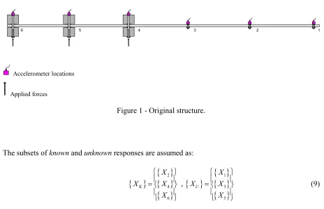
Figure 1 - Original structure.
The subsets of known and unknown responses are assumed as:
{ }
{ }
{ }
{ }
{ }
{ }
{ }
{ }
2 1
4 3
6 5
,
K U
X X
X X X X
X X
= =
(9)
The vector
{ }
F
A contains the loads which can be applied (even if some of them are null in certaincases)
{ }
{ }
{ }
{ }
4 5 6
A F
F F
F
=
(10)
According to eq. (5), and considering the above-defined subsets, the transmissibility matrix is given by:
12 14 16 14 15 16 24 25 26
32 34 36 34 35 36 44 45 46
52 54 56 54 55 56 64 65 66
(A) (A) (A)
(A) (A) (A)
(A) (A) (A)
T
T
T
H
H
H
H
H
H
T
T
T
H
H
H
H
H
H
T
T
T
H
H
H
H
H
H
+
=
(11)
3.2 Modified structures
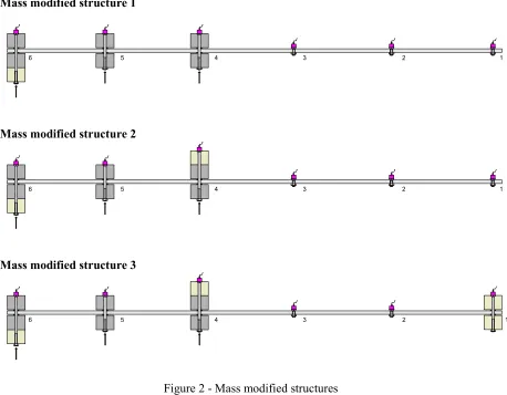
In order to prove that it is possible to obtain the FRFs in certain locations of modified systems, provided that the transmissibility matrix of the original system is known, some modifications have been made in the original structure. These modifications are made by adding masses or by changing the stiffness in certain regions.
The mass modifications made on the original structure are present in fig. 2 and the stiffness modifications in fig. 3.
5
Mass modified structure 1
6 5 4 3 2 1
Mass modified structure 2
6 5 4 3 2 1
Mass modified structure 3
[image:5.595.71.529.116.473.2]6 5 4 3 2 1
Figure 2 - Mass modified structures
Stiffness modified structure 4
6 5 4 3 2 1
Stiffness modified structure 5
[image:5.595.65.532.363.711.2]6 5 4 3 2 1
6
0 50 100 150 200 250 300 350 400
Frequency [dB] -160 -120 -80 -40 -180 -170 -150 -140 -130 -110 -100 -90 -70 -60 -50 R e c e p ta n c e [ d B ]
H14 (original structure) H14 (modified structure 1) H14 (modified structure 2) H14 (modified structure 3)
0 50 100 150 200 250 300 350 400
Frequency [dB] -160 -120 -80 -40 -180 -170 -150 -140 -130 -110 -100 -90 -70 -60 -50 R e c e p ta n c e [ d B ]
H14 (original structure ) H14 (modified structure 4) H14 (modified structure 5)
0 50 100 150 200 250 300 350 400
Frequency [Hz] -40 0 40 -30 -20 -10 10 20 30 50 60 M a g n it u d e [ d B ]
T52 (original structure) T52 (modified structure 1) T52 (modified structure 2) T52 (modified structure 3)
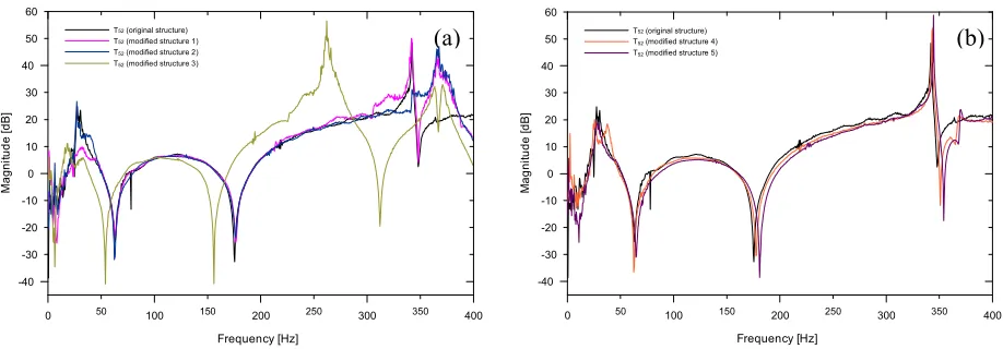
The measured receptances H14 are presented in fig. 4 for the various modified structures. Fig. 4a)
[image:6.595.74.529.173.316.2]shows the influence of the mass modifications, i. e., the decreasing of the natural frequencies, whereas in fig. 4b) it can be observed the influence of the stiffness modifications resulting in higher natural frequencies.
Figure 4: Measured receptances H14 for the original structure and modified structures:
a) mass modification, b) stiffness modification.
In figs. 5 and 6 two transmissibility functions, T52 and T32, respectively, are presented for the original
and modified structures.
Figure 5: T52 Transmissibility obtained for original structure and a) mass, b) stiffness modified
structures.
(a) (b)
(a)
0 50 100 150 200 250 300 350 400
Frequency [Hz] -40 0 40 -30 -20 -10 10 20 30 50 60 M a g n it u d e [ d B ]
T52 (original structure) T52 (modified structure 4)
[image:6.595.72.531.444.604.2]7
0 50 100 150 200 250 300 350 400
Frequency [Hz] -40 0 40 -30 -20 -10 10 20 30 50 60 M a g n it u d e [ d B ]
T32 (original structure) T32 (modified structure 1) T32 (modified structure 2) T32 (modified structure 3)
0 50 100 150 200 250 300 350 400
Frequency [Hz] -160 -120 -80 -40 -180 -140 -100 -60 R e c e p ta n c e [ d B ]
[image:7.595.74.525.94.253.2]H14(measured mod.1) H14(calculated mod.1) H35 (measured mod.1) H35 (calculated mod.1) H56 (measured mod.1) H56 (calculated mod.1)
Figure 6: T32 Transmissibility obtained for original structure and a) mass, b) stiffness modified
structures.
Remarks
It can be observed that in situations when the mass modifications on the original system are made on the values of the masses corresponding to the set of coordinates A (where the dynamic loads can be applied) the transmissibility values do not change, modified structures 1 and 2, figs. 5 and 6 (a). It can also be observed that when the modification on the original system is made on the stiffness region connecting co-ordinates of subset A the transmissibility values do not change, modified structures 4 and 5, figs.5 and 6 (b).
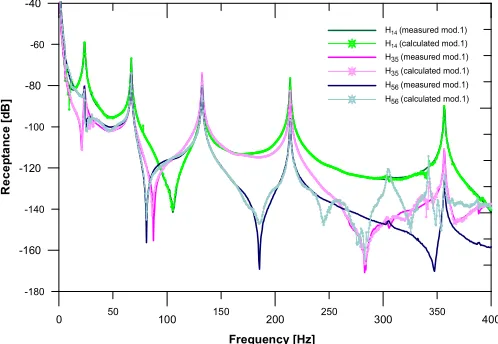
3.3 Estimation of FRFs using the Transmissibility concept
In figs. 7, 8, 9 and 10, three receptances ' 14
H , ' 35
H and ' 56
H , estimated for the modified structures 1, 2, 4 and 5, respectively, by using eq. (8), are presented and compared with the measured receptances on the actual modified structures.
Figure 7: Measured and estimated receptances H14 , H35 and H56 for the mass modified structure 1.
(a)
0 50 100 150 200 250 300 350 400
Frequency [Hz] -40 0 40 -30 -20 -10 10 20 30 50 60 M a g n it u d e [ d B ]
T32 (original structure) T32 (modified structure 4) T32 (modified structure 5)
[image:7.595.155.404.535.707.2]8
Figure 8: Measured and estimated receptances H14 , H35 and H56 for the mass modified structure 2.
0 50 100 150 200 250 300 350 400
Frequency [Hz] -160
-120 -80 -40
-180 -140 -100 -60
R
e
c
e
p
ta
n
c
e
[
d
B
]
H14(measured mod.4) H14(calculated mod.4) H35 (measured mod.4) H35 (calculated mod.4) H56 (measured mod.4) H56 (calculated mod.4)
9
0 50 100 150 200 250 300 350 400
Frequency [Hz] -160
-120 -80 -40
-180 -140 -100 -60
R
e
c
e
p
ta
n
c
e
[
d
B
]
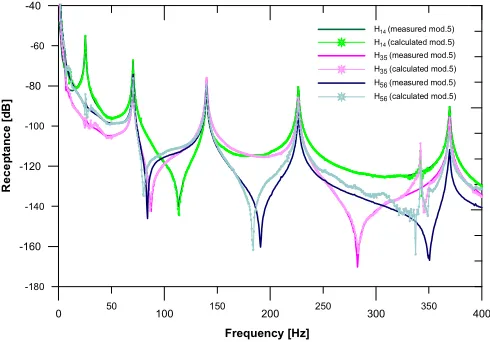
[image:9.595.175.420.131.302.2]H14(measured mod.5) H14(calculated mod.5) H35 (measured mod.5) H35 (calculated mod.5) H56 (measured mod.5) H56 (calculated mod.5)
Figure 10: Measured and estimated receptances H14 , H35 and H56 for the stiffness modified structure 5.
Remarks
It can be observed that the estimated FRFs of the various modified structures compare well with the FRFs measured on the actual modified structures. This is not the case for Receptance H56, mainly at
the anti-resonances as the frequency increases.
4
Conclusions
In this work it has been shown that it is possible to estimate the FRFs related to some points of interest that are not physically accessible. By using the important properties associated with the transmissibility matrix, obtained by measuring the FRFs at certain points due to some applied forces on an actual original structure, together with a set of FRFs measured on any modified structure, it is possible to estimate response data at certain inaccessible locations of different mass and stiffness modified systems.
Acknowledgements
The current investigation had the support of FCT, under the project PTDC/EME-PME/71488/2006.
References
10
[2] Varoto, P.S., McConnell, K.G., (1998), “Single Point Vs Multi Point Acceleration
Transmissibility Concepts In Vibration Testing”, Proc. of IMAC XVI, Santa Barbara, California, USA.
[3] Ribeiro, A.M.R., (1998), “On the Generalization of the Transmissibility Concept”, Proc. of the NATO/ASI Conference on Modal Analysis and Testing, Sesimbra, Portugal.
[4] Maia, N. M. M., Almeida, R. A. B., Urgueira, A. P. V., "Understanding Transmissibility Properties", Proceedings da 26th Conference and Exposition on Structural Dynamics (IMAC26), Orlando, Florida, USA, Fevereiro de 2008, paper 83.