ACOUSTIC PARTICLE VELOCITIES MEASUREMENT BY MEANS OF LASER DOPPLER VELOCIMETRY : APPLICATION TO HARMONIC ACOUSTIC FIELDS IN FREE SPACE WITH WEAK FLOW

ACOUSTIC PARTICLE VELOCITIES MEASUREMENT BY MEANS OF

LASER DOPPLER VELOCIMETRY : APPLICATION TO HARMONIC

ACOUSTIC FIELDS IN FREE SPACE WITH WEAK FLOW

Rouquier Philippe ; Gazengel Bruno ; Richoux Olivier ; Simon Laurent ; Tournois Guy ; Bruneau Michel

Laboratoire d’Acoustique de l’Université du Maine LAUM UMR CNRS 6613

Av. Olivier Messiaen 72085 Le Mans Cedex 09 France

Tel : 33 (2) 43 83 36 30 Fax : 33 (2) 43 83 35 20

E-mail :

[email protected]

ABSTRACT

A Laser Doppler Velocimeter is an optical measurement device used for estimating particle velocities, by means of specific signal processing of the light scattered by seeding particles. The velocimeter set-up we used has been adapted in order to measure acoustic particle velocities in gases. In previous works, specific signal processing methods have been developed for harmonic acoustic fields in ducts without flow. Then, the aim of this study is to measure the velocities of harmonic acoustic fields in free space with flow ; signal processing methods, estimating both flow and acoustic velocities, are presented, and their limits are discussed.

1. INTRODUCTION

Laser Doppler Velocimetry (LDV) is widely used for flow measurements but it may also be used for measuring the acoustic particle velocity [1]. The validation of its use for acoustics in a duct was being achieved [2] using both a commercial equipment originally dedicated to fluid mechanics, the Burst Spectrum Analyser 57N20 from DANTEC, and a system for acquisition and signal processing more specifically dedicated to acoustics, currently used and developed at the Laboratoire d'Acoustique de l'Université du Maine (LAUM). The aim of this study is the measure of velocities of harmonic acoustic fields in free space with weak flow. The harmonic acoustic source, a enclosed loudspeaker, takes place in a semi-anechoic room, and the weak flow is the natural air convection.

2. FUNDAMENTALS OF LASER DOPPLER VELOCIMETRY (LDV)

2.1Principle Of LDV

LDV is an optical technique allowing direct measurement of local and instantaneous particle velocity. Its principle is based on the determination of the Doppler shift of light scattered from seeding particles (tracers) suspended in the fluid. In the differential Doppler mode [4], two laser beams of equal intensity are focused and crossed at the point under investigation, forming an ellipsoidal volume consisting of equidistant dark and bright fringes called probe volume (figure 1).

fig. 1 : Optical Set-up of LDV system

When a tracer moves through this volume, the scattered light is making up an optical signal whose intensity is modulated at a frequency fD, called Doppler frequency, which is related to the velocity Vp, the particle tracer velocity along the x-axis, the fringe separation i, and the optical wavelength λL (see below).

The scattered light is collected on a photomultiplier (PM) whose output signal is called the Doppler signal. The PM can be located such that forward or backward scattering occurs. In forward scattering, the scattered light intensity is high and the signal to noise ratio (SNR) of the Doppler signal is high. For some applications, such as velocity measurements near walls, the back scattering mode can not be avoided ; its main drawback is that it provides a low quality Doppler signal due to the low intensity of the scattered light (about 100 times lower than the one collected in forward scattering). The PM output signal is then sampled and processed system in order to estimate the velocity parameters.

2.2 Doppler Signal Model

The Doppler signal collected on the PM can be modelled as a sine-wave modulation weighted by a gaussian shape depending on the tracer position xp(t) in the probe volume [2,4] :

(t)]},

x

i

2

cos[

{M

Ke

s(t)

2

p

π

β

+

=

with

L r

) 2 / cos(θ

=

β , the angle θ being the angle between the laser beams, The factor K is related

to the laser beam power, the PM sensitivity, the electronic amplification, the observation direction and the scattering efficiency of the tracer, and the length rL being the radius of the focused laser beams. The term e-[β xp (t)]²

represents the fringes envelope due to the Gaussian cross section of the laser beams. The corrective term M is due to the different intensities of the laser beams. If the particle velocity Vp remains constant while the particle crosses the probe volume, the Doppler signal take the form

)t]}.

2

sin(

V

cos[4

{M

Ke

t]}

i

V

cos[2

{M

Ke

s(t)

θ

λ

π

π

+

=

+

=

Equations 1 and 3 bring out a sign ambiguity since two particles crossing the probe volume with the same direction, the same velocity but opposite senses generate the same Doppler signal. Adding a frequency shift to one of the laser beams may solve the problem. This causes the fringe pattern to move. Particles moving in one direction will occur with a frequency higher than the added frequency shift, while particles moving in the other direction will occur with a frequency lower than the added frequency shift. In practice, the PM output signal is also frequency shifted down to the carrier frequency fc for adaptation to the signal processing. Consequently, equation 2 becomes

(t)]} x i 2 t f cos[2 {M Ke (t)

s_d -[ x (t)] _{c p}

2

p + π + π

= β .

In the case of acoustics measurements, the particle velocity inside the probe volume can not be assumed constant. Considering only purely sinusoidal waves, the particle velocity can be written

] t f Vcos[2

v(t)= π _exc +ϕ ,

where V and ϕ are respectively the amplitude and the phase to be measured, and fexc is the known driving frequency. The PM output signal can be written (see equation 4)

} )] t f 2 sin( t f cos[2 A(t){M (t)

s_d = + π _c +α π _exc +ϕ .

The amplitude A(t) can not be easily modelled unless the particle location in the probe volume is exactly known. However, preliminary tests performed by Valeau [3] have shown that, for acoustic particle velocity measurements, this amplitude remains almost constant during a few

periods of the acoustic signal. Furthermore, the modulation index α is defined by α= exc

ac if

V

, and

ranges, for example, from 0.96 to 19.34 for fexc = 1kHz and 1mm.s-1 < V < 20mm.s-1.

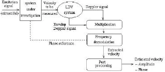
Equation 6 is valid only for one seeding particle crossing the probe volume. During the acquisition, several seeding particles cross nevertheless successively the probe volume. Each particle creates a so-called burst signal, each burst being described by equation 6. In the following, the measured velocities are supposed to be purely sinusoidal, since the excitation signal is sinusoidal and the system under investigation is linear. The principle of the signal processing used for extracting the velocity information consists in demodulating the frequency-shifted Doppler signal and analysing the frequency demodulated signal in order to estimate its amplitude and phase (figure 2).

fig 2 : General signal processing

(3)

(5)

(4)

Different techniques are used to perform the frequency demodulation. This present study focus on the use of the Short-Time Fourier Transform. This method gives an estimate of the instantaneous frequency (at the time corresponding to the middle of the window) from which the velocity is derived. Post-processing techniques described later in this paper are used to estimate the amplitude of the acoustic particle velocity.

3. Experimental set-up

The LDV device used in this study is a dual beam system operating in the differential Doppler mode. Only one velocity component is measured. The optical set-up is made of commercial equipment commonly used in fluid mechanics. Nevertheless, its arrangement has been modified as acoustic velocities differ significantly from flow velocities. First, all noisy equipment and heat sources are removed from the experimental room, in order to avoid as many external perturbations as possible and to preserve a sufficiently high signal to noise ratio of the Doppler signal. In order to get enough light intensity despite the back scattering configuration, a 1W argon laser is used. The laser source is set to operate in a single mode, producing a 514.5nm wavelength in air. Furthermore, as the acoustic particle velocity amplitudes are much lower than those of flow velocities, the sensitivity of the system has to be enhanced. This is done increasing the angle between the two incident beams : it is set to 28.87° instead of a few degrees for flow measurements. The interference network counts 120 fringes. As previously discussed, the velocity sign discrimination requires the use of a Bragg cell, introduced on the path of one of the incident beams. The Bragg cell operates here in the –1 mode, which lowers the frequency of the beam that is frequency shifted. The cell is driven at fB=40MHz.

The aim of this experiment is the simultaneous estimation of acoustic particle velocities and flow velocities. For the experiments presented in this paper, the acoustic source is an enclosed loudspeaker, the flow source is the natural convection, and the experience takes place in a semi-anechoic room. Thanks to this experimental conditions, the acoustic particle velocity Vac can roughly be predicted by an acoustic pressure measurement Pac, using the following equation

ac

ac cV

P =ρ ,

where ρ the density and c the sound velocity in the air.

4. Signal processing techniques

The signal acquisition system performs frequency demodulation with the help of a custom software. Once the Doppler signal has been frequency shifted thanks to the Bragg frequency (40 MHz) to a new carrier frequency fc, the Doppler signal is low pass filtered with the help of a Bessel filter having a linear phase in the frequency range of interest. The filtered signal is sampled at a sampling rate FsAcq. This sampling frequency is chosen such that the Shannon theorem is fulfilled. In practice, the signal is oversampled by choosing a high sampling frequency. A Short Time Fourier Transform (STFT) is applied using sliding windows (Kaiser windows) which can overlap in time. For each window of Nw samples, a FFT enables to estimate the frequency content of the frequency shifted Doppler signal. Thus, point to point, a frequency signal, so-called instantaneous frequency fi(t), is calculated. This instantaneous frequency fi(t) is related to the particle velocity Vp(t) by equation

) t f 2 cos( V f * i ) t ( f * i ) t (

V_p = _i = _c+ _ac π_exc +ϕ_ac .

In this experiment, the particle velocity is the sum of flow velocity and acoustic particle velocity. Each velocity is estimated by signal processing: the flow velocity Vc, included in the carrier velocity i* fc, is estimated from the particle velocity signal average ; the acoustic particle velocity, whose frequency fexc is known, is estimated using a synchronous detection. Thanks to this signal processing techniques, two others parameters can be estimated : the acoustical signal to noise ratio (SNR), i.e. the power of acoustic contribution divided by the power of

non-(7)

acoustic contribution, and the tracer volume probe crossing date tk. The dates tk bring out information about tracers properties. Lastly, four parameters are estimated.

5. Results : Acoustic Field with natural convection flow

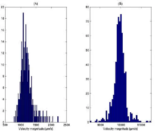
The experiments were done using three acoustics frequencies fexc (500Hz, 1000Hz and 2000Hz) and three sound pressure levels (approximately 80dB, 90dB and 100dB SPL, measured by mean of a microphone). For each experiment, around one thousand bursts are acquired, and the four parameters described previously (Vac, Vc, tk, SNR) are determinate for each of them. Thus, the numerous data allow statistical studies, such as histogram, as shown in figure 4 for acoustic particle velocity, and in figure 3 for flow velocity.

Fig. 3 : Histograms of flow velocity for an acoustic frequency fexc = 2000Hz. (A) : acoustic level equal to 80 dB SPL ; (B) : acoustic level equal to 100 dB SPL

Fig. 4 : Histograms of acoustic particle velocity for an acoustic frequency fexc = 2000Hz. (A) : acoustic level equal to 80 dB SPL ; (B) : acoustic level equal to 100 dB SPL

80 dB SPL 90 dB SPL 100 dB SPL

Vac ∆Vac VPred. Vac ∆Vac VPred Vac ∆Vac VPred

500Hz 0.69 0.31 0.72 2.11 0.37 2.15 6.4 0.37 7.06

1000Hz 0.89 0.47 0.83 2.64 0.41 2.49 8.12 0.31 7.96

2000Hz 1.15 0.41 0.86 3.33 0.47 2.55 9.95 0.58 8.13

Table 1 : acoustic particle velocity results (in mm.s-1)

80 dB SPL 90 dB SPL 100 dB SPL

Vc ∆Vc Vc ∆Vc Vc ∆Vc

500Hz 0.29 16.71 -0.5 17.74 -4.75 18.76

1000Hz -1.98 19.95 -2.34 19.05 -11.77 17.00

2000Hz -2.99 23.04 1.57 18.57 -10.37 16.06

Table 2 : flow velocity results (in mm.s-1)

where Vac (respectively Vc) is the estimated mean acoustic particle velocity (respectively the flow velocity) (expressed in mm.s-1), ∆Vac the 95% confidence interval of Vac(t) (respectively Vc(t)) (expressed in mm.s-1) and VPred the predicted acoustic particle velocity (expressed in mm.s-1), determined with the help of equation (7).

For a given acoustic pressure level, the acoustic frequency does not seem to have influence on the precision of the acoustic particle velocity estimation. As example, for an acoustic pressure level equals to 100dB SPL, the relative precision (∆Vac/ Vac) is nearly 5-6%. As expected, for a given acoustic frequency, the precision on the estimated acoustic particle velocity is higher for 100 dB SPL than for 80 dB SPL. As example, the relative precision for fexc=2000Hz is nearly 6% at 100dB SPL, whereas the relative precision for fexc=2000Hz is nearly 36% at 80dB SPL. Indeed, for high acoustic pressure level, acoustic particle velocity is of about size of flow velocity, which is considered as noise. So the measure precision is higher for high acoustic pressure level than for low acoustic pressure level. However, for low acoustic pressure level, the results remain quiet good, as shown by the comparison between the acoustic particle velocity measured by VLD and the acoustic particle velocity estimated by a pressure measurement. The presence of a flow does not seem to prevent the acoustic particle velocity measurement, even if the level of noise disturbs the estimation.

In this paper, the weak flow is only characterised by means of its mean flow velocity. The estimation of other parameters, such as power spectral density, are expected in future works. As shown in figure 3 and table 2, the acoustic pressure level and the acoustic frequency seem to have influence on the mean flow velocity value. However, because of different seeding conditions, the experimental conditions, in particular the number of data, are different from one experiment to an other, which can also explained the different mean flow velocity. The influence of each parameter (acoustic frequency, acoustic pressure level and experimental conditions) is the aim of the future experiments.

REFERENCES

[1] TAYLOR K.J. "Absolute measurement of acoustic particle velocity" J. Acous. Soc. Am. 1976; 59(3) : 691-694.

[2] Poggi S. "Contribution au developpement d'un banc de mesure de la vitesse particulaire acoustique par vélocimétrie laser Doppler (VLD) : evaluation des resultats et application" Ph. D. Thesis, université du Maine, 2000.

[3] Valiere J.C., Herzog P., Valeau V., Tournois G. "Acoustic velocity measurements in the air by means of Laser Doppler Velocimetry : dynamic and frequency range limitations and signal processing improvements" J. Sound. Vib., 229(3), 607-626, 2000.