A Study on analysis of intracranial acoustic wave propagation
by the finite difference time domain method
43.35 Wa Biological effects of ultrasound, ultrasonic tomography
Yoko Tanikaga, Toshikazu Takizawa, Takefumi Sakaguchi, Yoshiaki Watanabe
Faculty of Engineering, Doshisha University
1-3, Tataramiyakotani, Kyotanabe-shi
610-0321 Kyoto
Japan
81-774-65-6712
81-774-65-6300
dtb0176@mail4.doshisha.ac.jp
ABSTRACT
To find out the sensory mechanisms of the bone-conducted ultrasound, the propagations of intracranial acoustic are simulated by the finite difference time domain (FDTD) method. Elastic wave propagation in some models consisting of solid and liquid are studied experimentally and numerically and it is confirmed that both two results are agreed well. The sound field of intracranial acoustic wave are also studied and it is shown that some interesting results are obtained concerned with the peripheral part in the sensory mechanisms.
INTRODUCTION
hand, the powerful calculation tool of the finite difference time domain (FDTD) method have been developed and applied to the sound field. In this report, to find out the mechanisms, the simulation of intracranial acoustic wave propagations is tried by the FDTD method. Firstly, to examine the validity of the FDTD method, the propagations of elastic wave in some models consisting of a homogeneous solid and liquid are studied numerically by the elastic-FDTD method including both the longitudinal and transverse waves. Then experimental studies were also carried out using the same models and compared with the calculated results. Finally, intracranial sound fields are performed by the acoustic-FDTD method considering just the longitudinal wave, and the sensory mechanisms are discussed based on the calculated results.
OUTLINE OF THE FDTD METHOD
The sound wave in a 2-dimensional sound field is described by the following differential equations. Equations (1) and (2) show the generalized Hooke’s law in x- and y- directions, respectively, Eq. (3) shows the displacement and distortion, and Eqs. (4) and (5) show the motion in x- and y- directions, respectively.
xx NS y x
xx
y v
x v
t λ µ λ η σ
σ −
∂ ∂ + ∂ ∂ + = ∂ ∂
) 2
( (1)
yy NS y x
yy
y v x
v
t λ λ µ η σ
σ −
∂ ∂ + + ∂ ∂ = ∂ ∂
) 2
( (2)
xy SS y x xy
xy
x v y v t
t µ η σ
σ
σ −
∂ ∂ + ∂ ∂ = ∂ ∂ = ∂
∂ (3)
∂ ∂ + ∂ ∂ = ∂ ∂
y x t
vx σxx σxy
ρ
1 (4)
∂ ∂ + ∂ ∂ = ∂ ∂
y x t
vy σxy σyy
ρ
1 (5)
where,
σ
ij is the stress tensor,v
i is the particle velocity,ρ
is the density,η
NS andη
SS are absorption loss coefficients for the longitudinal and transverse waves respectively, andλ
andµ
are the Lame’s constants. These 5 equations are approximated by the centralfinite difference in the time and space domain. An initial condition is given to the stress tensor of longitudinal wave, the particle velocity is calculated and the stress tensor is calculated step by step. The spatial distributions of sound pressure are visualized by using calculated results.
COMPARISON BETWEEN CALCULATIONS AND EXPERIMENTS
Calculation Conditions
calculated sequentially in a time step of 0.01
µ
s
. As the boundary condition of analysis areas, the 2nd-order Higdon boundary operator was accommodated on the boundaries to make them non reflective. The sound source was assumed to be a group of point sources within a space of 10 mm, to be perfectly reflective and to have the piston action. The values used in the calculation are shown in Table 1. As the initial condition, a single sinusoidal wave of 1 MHz is set to the stress tensors (σ
xx andσ
yy). [image:3.596.94.504.180.324.2]Fig.1 Samples of acrylic resin (a) a flat plate (b) a cylinder.
Fig.2 Spatial models of (a) a flat plate (b) a cylinder.
Table 1 Acoustic constants.
Experimental Conditions
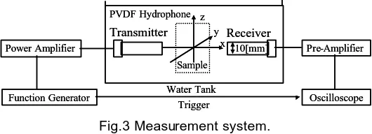
To examine the validity of calculation the FDTD method, an experiment was performed using the observation system as shown in Fig. 3. A water tank was filled with degassed water. A transmitter and a receiver were placed facing each other and the sample were put between them. The distance between the transmitter and receiver was set to 100 mm for the flat plate and 70 mm for the cylinder. The flat plate was rotated about the z-axis as shown in Fig. 1. As same as the calculated initial condition, a single sinusoidal wave with of 1 MHz was generated, then the transmitted waves through the sample are picked up by the receiver.
Fig.3 Measurement system.
Results of Calculation and Experiment and Discussion
Figure 4(a) and 5(a) show the observed waveforms when
θ
= 0oandθ
= 20o, respectively. These waveforms are normalized by the maximum amplitudes. In this figures,is the wave that travels straight through the acrylic and is the wave that is reflected two times. Many waves were observed in the condition of
θ
= 20o, however some of these waves cannot(a) (b)
x z
300[
mm]
25.8[mm] 30.0[mm]
x
Į
10[mm]
40[mm]
z
40[
mm]
y
y
(a)
(b)
Y
10.0 10.0
100.0
60.0
40.0
10.0
Transmitter Receiver
[mm]
Y
X
10.0 15.0 10.0
12.9
70.0
Transmitter
Receiver 35.0 [mm]
X
(a)
(b)
Y
10.0 10.0
100.0
60.0
40.0
10.0
Transmitter Receiver
[mm]
Y
X
10.0 15.0 10.0
12.9
70.0
Transmitter
Receiver 35.0 [mm]
X
Pre-Amplifier
Trigger z PVDF Hydrophone
Transmitter Receiver
Water Tank x
Sample
10[mm] y
Power Amplifier
Function Generator Oscilloscope
Pre-Amplifier
Trigger z PVDF Hydrophone
Transmitter Receiver
Water Tank x
Sample
10[mm] y
Power Amplifier
Function Generator Oscilloscope
Water Acrylic
Sound Velocity of Longitudinal Wave[m/s]
Sound Velocity of Transverse Wave[m/s]
Density [kg/m ]3 1000
1483 ----0.025
----Absorption Loss for Longitudinal Wave[neper/m]
Absorption Loss for Longitudinal Wave[neper/m]
1180 2729 1729 16.0 45.0
Water Acrylic
Sound Velocity of Longitudinal Wave[m/s]
Sound Velocity of Transverse Wave[m/s]
Density [kg/m ]3 1000
1483 ----0.025
----Absorption Loss for Longitudinal Wave[neper/m]
Absorption Loss for Longitudinal Wave[neper/m]
[image:3.596.165.430.580.676.2]be appeared when
θ
= 0o. The waves, , , and , appeared as a result of mode conversion and propagation by transverse waves in the acrylic. The polarity reversal is observed in . Figures 4(b) and 5(b) show the calculated waveforms by FDTD method. The calculated results are agreed well with the observed results in both the conditions. It is also found the appearance time, the amplitudes, and the polarity of waves are well simulated. However the small ringing phenomena are appeared in the calculated results.Fig.4 Waveforms traveling through the acrylic flat plate for = 0 deg. (a) observed waveform (b) calculated waveform.
Fig.5 Waveforms traveling through the acrylic flat plate for = 20 deg. (a) observed waveform (b) calculated waveform.
Figure 6(a) shows the observed waveform in the case of cylindrical sample. The waveform was normalized by the maximum amplitude. In this figure, is the wave that travels straight through the acrylic, is the wave that travels through the acrylic with a reflection two times between the acrylic cylinder and the surface of the transmitter, and is the wave that travels through with a reflection two times in the acrylic cylinder.
[image:4.596.86.506.610.747.2]Figure 6(b) shows the calculated waveforms by the FDTD method. The calculated results are also agreed well with the waveforms. However the small differences are found between the observed and the calculated waveform in the some parts of waveforms.
Fig.6 Waveforms traveling through the acrylic cylinder.
(a) observed waveform (b) calculated waveform. The followings are given to explain the difference.
1.0
0.5
0.0
- 0 . 5
Amplitude[V]
8 5 8 0 7 5 7 0 6 5 6 0
T i m e [ ƒÊ s] (a)
‡ @
‡ B
- 0 . 8 - 0 . 4 0.0 0.4
Amplitude[V]
8 5 8 0 7 5 7 0 6 5 6 0
T i m e [ ƒÊ s] (b)
‡ @
‡ B
0.4
0.0
- 0 . 4
Amplitude[V}
8 5 8 0 7 5 7 0 6 5 6 0
T i m e [ ƒÊ s ]
( a )
‡ @
‡ A
‡
B ‡C ‡D
- 0 . 6 - 0 . 4 - 0 . 2 0.0 0.2
Amplitude[V]
8 5 8 0 7 5 7 0 6 5 6 0
T i m e [ ƒÊ s ]
( b )
‡@ ‡
A ‡B ‡C
‡ D
1 . 0
0 . 5
0 . 0
- 0 . 5
Amp
litude[V]
1 0 0 9 0 8 0 7 0 6 0 5 0 4 0
T i m e [ ƒÊ s ]
‡ @
‡ A
‡ B ( a )
- 0 . 8 - 0 . 4 0 . 0 0 . 4
Amp
litude[V]
1 0 0 9 0 8 0 7 0 6 0 5 0 4 0
T i m e [ ƒÊ s ]
‡ @
‡
A ‡B
(a) The value of absorption loss in the numerical calculation was not suitable.
(b) The initial waves used in the calculation was different from actual waves according to the transitional characteristic of the transducers.
(c) The surface of transmitters did not vibrate uniformly.
CALCULATION OF A HUMAN’S HEAD MODEL
Calculation
In this section, the intracranial sound field is discussed. Human’s head is consisted of solid and liquid, so that both the effects of longitudinal and transverse waves have to be considered. However, it is necessary to know the absorption effects of the transverse wave for the exact estimation in the elastic-FDTD method. But the absorption loss in the brain is not clear in wide frequency range, so the acoustic-FDTD method is used in this report.
[image:5.596.121.480.406.512.2]As shown in Fig. 7, the heterogeneous head model [1] was consisted of seven tissues, bone, brain, muscle, eye, fat, skin and lens. The model of cell size was 2.5 mm and the number of lattice was 100 in length, 100 in width and 110 in height. The transducer of 10 mm in diameter was set near the left ear of the head model and the stimuli of the bone-conducted ultrasound is simulated. It is calculated sequentially in a time step of 0.25
µ
s
. The tissues were classified into two groups, bone and the others as soft tissue. Acoustic constants used in the calculation are shown in Table 2 [2][3]. The acoustic source was continuous sinusoidal waves of 3-40 kHz. To avoid the ringing effects, the lamp function is multiplied to the starting phase of 5 or 10 waves.Fig. 7 The heterogeneous head model of
(a) the sagittal slice, (b) the coronal slice, and (c) the transverse slice.
Table 2 Acoustic constants.
Results and Discussion
Figure 8(a)-(f) show the distribution maps of maximum sound pressure at the xy-plane including cochlear when the left side of the ear is stimulated in some frequencies. In the case of the frequencies are 3 kHz and 10 kHz, the peak of sound pressure was observed at the same side of stimuli. However when the stimulated frequencies were set over 15 kHz, the peak of sound pressure was found not only the same side but also at the opposite side of stimuli, and the distribution of sound pressure show the complex patterns. A wavelength is shorter than 100 mm when the frequency is over than 15 kHz, so the size of the parts cannot be ignored to the wavelength, so that spatial the distribution of sound pressure was complicated. It is thought that
Bone Soft Tissue
Volume Elasticity [Pa]
Density [kg/m ]3 1.70× 10
1.62× 10
1.05× 10 2.24× 10
3 3
9 1 0
Bone Soft Tissue
Volume Elasticity [Pa]
Density [kg/m ]3 1.70× 10
1.62× 10
1.05× 10 2.24× 10
3 3
9 1 0
top
2
3 5
1
(a) top
1 2
3 6
(b ) right
4 2 5 (c) top
2
3 5
1
(a) top
2
3 5
1
(a) top
1 2
3 6
(b ) top
1 2
3 6
(b ) right
4 2 5
(c) right
4 2 5 (c)
[image:5.596.184.401.574.618.2]the movement phenomena of sound images, reported in the bone-conducted ultrasound [4], can be expressed by the presented calculation results.
Fig. 8 Spatial distribution of intracranial sound pressure for (a) 3 kHz, (b) 10 kHz, (c) 15 kHz, (d) 20 kHz, (e) 25 kHz and (f) 30 kHz.
CONCLUSIONS
Some examples of sound field simulation based on the numerical calculation using the FDTD method were presented. These calculated results can be demonstrated much more effectively by computer simulation. It is recognized that calculated such a simulation technique may contribute to intuitive understanding the sensory mechanism of the bone-conducted ultrasound.
BIBLOGRAPHICAL REFERENCES
[1] O. Fujiwara and A. Kato, “Computation of SAR inside eyball for 1.5-GHz microwave wxposure using finite-difference time-domain technique,” IEICE Trans. Commun., xol.E77-B, no.6, pp732-737, 1994.
[2] J.C.Lin, “On microwave-induced hearing sensation,” IEICE Trans. Microwave Theory Tech., vol.MTT-25,no.7, pp.605-613,1977.
[3] V.K. Goel, H. Park, and W. Kong, “Investigation of vibration characteristics of the ligamentous lumbar spine using the finite element approach,” Trans. ASME, J. Biomechanical Engineering, vol.116, pp.377-383, 1994.
[4] T. Sakaguchi, “Study of perception by the bone-conducted ultrasound” Technical report of IEICE US98-93 1999 (in Japanese).
(f) (e)
(d)
(c) (b)
(a)
(f) (e)
(d)
(c) (b)