PREDICTION OF EXCESS ATTENUATION OF ROAD TRAFFIC NOISE BY DETACHED HOUSES

PREDICTION OF EXCESS ATTENUATION OF ROAD TRAFFIC NOISE

BY DETACHED HOUSES

PACS: 43.50.Rq

Anai, Ken; Fujimoto, Kazutoshi

Department of Architecture and Urban Design, Faculty of Human-Environment Studies Kyushu University

6-10-1 Hakozaki, Higashi-ku 812-8581 Fukuoka

JAPAN

Tel: +81 92 642 3338 Fax: +81 92 642 4113

E-mail: anai@arch.kyushu-u.ac.jp (K. Anai); fujimoto@arch.kyushu-u.ac.jp (K. Fujimoto)

ABSTRACT

The purpose of this paper is to present a simple method to predict excess attenuation of road traffic noise by detached houses. ASJ shows one method, but it cannot estimate the noise level at specific individual points in a residential area. So in this paper, a one-twentieth scale model experiment is performed and a new empirical formula for excess attenuation based on only five parameters is proposed. The validity of it is verified by comparison with additional experiment, a current method and noise measurements. This method is applicable to the evaluation of the environmental quality standards for noise.

INTRODUCTION

In Japan, residential areas often adjoin arterial roads because Japan is a small country. Residential buildings in such areas are seriously affected by road traffic noise, and the countermeasure to road traffic noise must be solved immediately. On such a background, the Ministry of Environment in Japan revised 'Environmental Quality Standards for Noise' [1] and enforced it in 1999. In it, an achievement of environmental noise in areas facing roads is evaluated by obtaining numbers and rates of the buildings at which noise levels exceed environmental quality standards regarding the respective concerned areas. The standard also admits estimating the noise level instead of actual measurement in case measurement is difficult. In order to estimate noise level, it is necessary to grasp excess attenuation by buildings. But it is very difficult to deal noise propagation rigorously in a residential area where more than one complex shape buildings are located. Uesaka et al. [2] showed a method of estimating 'average' noise level behind buildings, which was adopted into 'Acoustical society of Japan's Prediction Model 1998 for Road Traffic Noise (ASJ Model 1998)' [3]. In addition to this, predicting noise attenuation at a 'specific point' and estimating the distribution of noise level in a residential area is significant and effective for evaluating actual environment.

SCALE MODEL EXPERIMENT

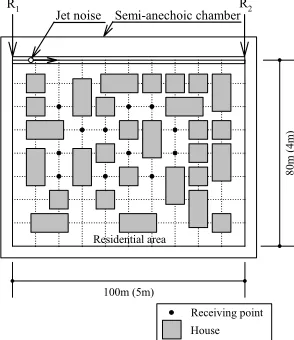
Outline Of Experiment One-twentieth scale model of a residential area that was 100m*80m (original size), as shown in Fig. 1, was set in a semi-anechoic chamber and the sound pressure level (Lp) was measured at receiving points in a residential area when a model vehicle ran a

straight road with a length of 100m. Then excess attenuation of road traffic noise by detached houses was calculated.

Model Houses Each detached house was assumed to be a rectangular parallelepiped with a size of 8m*8m or 8m*16m in ground plan and with a height of 4, 7 or 10m, and to be placed in the residential area at random. The ratio of the area of houses to whole residential area (hereafter, 'covering percentage') was set to four stages that are 16.8, 21.6, 28.0 or 34.4% as shown in Fig. 2. The model houses were made of polystyrene that was reflective in the frequency range of the measurement.

Model Source And Receiving Points Jet noise was used for a model sound source. The frequencies of it cover the range from 200 to 1,600Hz (original scale) for road traffic noise and it could be considered to be an omni-directional point source in those frequencies. The height of source was 0.5m from the ground. Measured Lp at each receiving point was converted into

A-weighted sound pressure level (LpA) by using a digital filter when assuming that a model

source have the spectrum of road traffic noise [6]. The number of receiving points was 12 shown in Fig. 1. The distances between the receiving points and the straight road (d) were 20, 30, 40, and 50m, and the height (hp) from the ground was 1.2, 5.2, and 8.2m. Here, the height of all

receiving points was under the height of houses for the reason mentioned below.

Excess Attenuation The sound exposure level (LAE) was calculated from the unit pattern that was

time-change of the noise level measured at the receiving point while the source moved from one end (R1) to the other (R2) on the straight road. And excess attenuation by houses (∆LAE) was

defined by a subtraction of LAE1 from LAE0, where LAE1 and LAE0 were the values of LAE measured

in the conditions that houses were placed and not placed respectively. A notice should be taken that the excess attenuation defined here has a contrary sign to usual definition.

DERIVATION OF PREDICTION FORMULA

Parameters For Prediction Since this study aims for a simple method to predict excess attenuation of road traffic noise by detached houses, parameters for prediction formula must be simple. As a result, five parameters were introduced. Two parameters among them are based on a given isosceles triangle with a vertex angle of 2π/3 (hereafter, 'base triangle'), the vertex of which is a predicting point and the base side of which is a road as shown in Fig. 3. One is the summation of angles decided by the roads that are visible from the receiving point as shown in Fig. 3 (hereafter, 'open angle' _φ). The _φ is 2_π/3 when no house is placed and zero when the road

100m (5m)

80

m (

4m)

Receiving point

Jet noise Semi-anechoic chamber

R1 R2

House Residential area

Fig. 1. Outline of the model experiment

T-13, T-23, T-33

T-11, T-21, T-31 T-12, T-22, T-23

T-14, T-24, T-34

is not visible at all. Another is a rate of the total housing area of the base triangle to the base triangle area (hereafter, 'house-occupied rate' _ξ).

If receiving point is higher than houses, a case when the road is visible over the houses from the receiving point happens. In such a case, the ξ defined above cannot present an exact open angle. In this research, therefore, the height of receiving points is limited to be smaller than the height of houses. Other three parameters are the distance between a receiving point and a road (d), the height of houses (H) and the height of a receiving point (hp).

Relation Between ∆LAE And φ Or ξ Since excess attenuation is not affected so much by houses

when the road is visible [4,5], the relation between ∆LAE and φ was firstly examined when φ is not

zero. The results are shown in Fig. 4. It can be found that ∆LAE decreases as φ decreases and its

relation dependents on H, hp and d. The relation between ∆LAE and φ was expressed with a*log10

(3_φ/2_π (1–b)+b) in each d, H and hp and the regression coefficients were calculated by the least

square method. Then, coefficients a and b were expressed with a function of d, H, and hp.

Next, the effect of ξ on the difference between ∆LAE and a*log10 (3φ/2π (1–b)+b) was examined,

because excess attenuation is affected by houses when the road is not visible [4,5]. The result shows that ∆LAE decreases as ξ increases and d, H and hp influence on ∆LAE hardly. So the

difference between ∆LAE and a*log10 (3φ/2π (1–b)+b) was firstly expressed with an equation of

u*_ξ+v, and then regression coefficients u and v were calculated.

Empirical Formula Thus, an empirical formula to predict excess attenuation of road traffic noise by detached houses was obtained as follows:

(

)

{

}

(

)

(

)

φ _φ

ξ φ

≠ π

=









10 AE

10

3

a * log 1- b + b , 0

∆ = 2

a * log b + u + v, 0

L (1)

where

∆LAE: excess attenuation by detached houses (dB)

φ: open angle (rad.)

ξ: house-occupied rate (-)

d: distance between a receiving point and a road (m) a: a = p+q*log10 d

p: p = 2.03H – 2.63hp + 4.64

q: q = – 1.10H + 1.47hp – 1.21

b: b=10(sd+t)/a

s: s = – 0.0023H – 0.009hp – 0.123

t: t = – 0.29H + 0.94hp – 3.74

u: u = –20.0 v: v = 6.59

H: height of houses hp: height of receiving point

Because of the experimental conditions, the formula is valid only when d is within 50m from a road, _ξ is less than 0.4, H is within 10m and hp is less than the height of houses. The comparison

between the experimental values and the predicted ones by equation (1) is shown in Fig. 5. The correlation coefficient between them is 0.95, and the differences between them are within ±3dB. So the prediction formula has a sufficient accuracy.

EXAMINATION ON VALIDITY OF PREDICTION FORMULA

Verification By Experiments In order to verify the proposed formula, two kinds of additional model experiments were performed.

In the first experiment, the experimental conditions were the same as in the former one except hp.

or 6.2m when H was 7m, and 3.2, 6.2, or 9.2m when H was 10m. As a result of the examination, it was found that the correlation coefficient between the experimental values and the predicted ones was 0.93, and the differences between them are within _±3dB. This verifies that the proposed formula has a sufficient accuracy even when hp is varied.

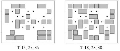
In the second experiment, not only hp but also housing arrangement was changed. Employed

new arrangements of houses are shown in Fig. 6. The covering percentages were 24.8% on T-x5 (x= 1, 2 and 3) and 32.8% on T-x8 (x=1, 2 and 3), which were in the coverage of the prediction formula. The hp was 1.2 or 3.2m when H was 4, 1.2, 3.2, 5.2, 6.2 or 7.0m when H was 7m, and

1.2, 3.2, 5.2, 6.2, 8.2 or 9.2m when H was 10m. As a result of the examination, it was found that the correlation coefficient between the experimental values and the predicted ones was 0.84, and the differences between them were roughly within ±3dB. This verifies that the formula has a sufficient accuracy even when hp and housing arrangement are varied.

ASJ Model 1998 The prediction formula was compared with the method to predict the attenuation by buildings shown in ASJ Model 1998. The housing arrangements T-x1, T-x2, T-x3 and T-x4 (x=1, 2 and 3) shown in Fig. 2 were used for the comparison. ASJ Model 1998 aims to predict the average value in evaluating region, and consequently it represents the same value when the distance from a road is constant. On the other hand, the proposed formula predicts the attenuation at a specific point. For the comparison, the attenuations at the points at intervals of 1m on seven lines (from 20 to 50m at intervals of 5m) parallel to a road were calculated by equation (1). Then the arithmetic average value on individual line was compared with the value predicted by ASJ Model 1998. An example of the results is shown in Fig. 7. Equation (1) represents a little small value compared with ASJ Model 1998 while the receiving point parts from the road, but the differences between them are not so much.

As mentioned above, the prediction formula provides an individual value at each predicting point even while ASJ Model 1998 does only the average value in the whole target area. The degree of the agreement between the proposed formula and ASJ Model 1998 strongly depends on the arrangement of houses. Therefore Fig. 7 is only an example.

Road

φ 1 φ 2 φ 3

2π/3

P φ = φ1+φ2+φ3

Fig. 3. Base triangle and open angle φ

d = 20m

0.0 0.5 1.0 1.5 2.0 2.5

∆

L

AE

(dB

)

-20 -15 -10 -5 0

5 d = 30m

0.0 0.5 1.0 1.5 2.0 2.5 -20

-15 -10 -5 0 5

d = 40m

φ (rad)

0.0 0.5 1.0 1.5 2.0 2.5

∆

L

AE

(d

B

)

-20 -15 -10 -5 0

5 d = 50m

φ (rad)

0.0 0.5 1.0 1.5 2.0 2.5 -20

-15 -10 -5 0 5

Fig. 4. Relation between _∆LAE and φ (H=10m, hp=1.2m)

Predicted ∆LAE(dB)

-20 -15 -10 -5 0 5

Me

as

ure

d

∆

L

AE

(dB)

-20 -15 -10 -5 0 5

+ 3dB

- 3dB N=288

Fig. 5. Comparison between measured values and predicted ones by equation (1)

T-18, 28, 38 T-15, 25, 35

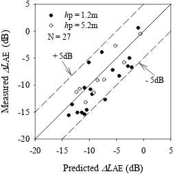
Noise Measurement In Actual Area Road traffic noise was measured at two actual residential areas (areas A and B) along roads with heavy traffic. In order to obtain excess attenuation by houses, LAeq during 20s was measured at the points both by road side and in the residential area

simultaneously. The numbers of the measuring points by road side were 2 in A and 3 in B, and the points in the residential area were 15 in A (9: hp=1.2m and 6: hp=5.2m) and 12 in B (9:

hp=1.2m and 3: hp=5.2m). Excess attenuation ∆LAE was calculated by the following formula; ∆LAE

= LAE,d – LAE,d0 + 10* log10 (d/d0), where LAE,d is a measured value in the residential area and

LAE,d0 is one by road side, and d0 and d are the distances between the measuring point by road

side and in the residential area and the center of the road respectively. Fig. 8 shows the comparison between the measured value and the predicted one by equation (1). The differences between them are within ±5dB when hp is 1.2m and within ±3dB when hp is 5.2m. It can be said it

is a good agreement on the whole.

It is guessed that the reason why the measured values tend to be moderately smaller than the predicted ones when hp is 1.2m is caused by a guardrail, a wall, and garden plants which are not

drawn on a map.

APPLICATION OF PREDICTION FORMULA

In order to confirm an application of the prediction formula, simulations for the noise level distribution in a residential area were performed. Housing arrangement T-32 (H=10m) in the former experiment was used for the simulation. Fig. 9 shows some examples of noise distribution. In the ground plan, the height of receiving points is 1.2m. Here the noise level LpA at the point

with a distance of d from the center of a road was calculated by an equation LpA = LWA – 8 –

10*log10 d + ∆LAE + ∆Lg, where LWA shows A-weighted sound power level of road traffic noise

(dB/m) and _∆Lg shows compensation of effect by ground surface. That is, LpA shows the relative

value by substituting 0dB/m for LWA, and 3dB for ∆Lg as a semi-free sound field. Since equation

(1) can predict excess attenuation at arbitrary points which are lower than houses, the noise level distribution not only on the fixed height but also in the perpendicular direction can be grasped.

Fig. 10 shows an example of the noise distribution when the houses are not randomly arranged. In this simulation, the height of houses is 7m and the height of receiving points is 1.2m. The contour line calculated by ASJ Model 1998 is parallel to a road in a plane distribution chart. On the other hand, the prediction formula provides the reasonable noise distribution corresponding to arranged houses because it can predicts an individual value at each predicting point. Especially in the zone with a wide view of the road, remarkable difference is recognized between them.

CONCLUSION

A one-twentieth scale model experiment was performed and a simple method for predicting excess attenuation of road traffic noise by detached houses was proposed. This method can predict excess attenuation at arbitrary points below the height of houses. The validity and accuracy of the proposed formula were verified by two additional experiments, comparison with ASJ Model 1998 and noise measurements in actual residential areas. And it was shown that the proposed formula could provide the distribution of noise level corresponding to arranged houses. Since five parameters used in the formula, the open angle (_φ), the house-occupied rate (_ξ), the distance between a receiving point and a road (d), the height of houses (H) and the height of a receiving point (hp), can be easily obtained at the beginning stage of planning for residential

areas, the formula can be applied to a planning of housing arrangement in a residential area with considering the effect of road traffic noise.

BIBLIOGRAFICAL REFERENCES

[1] Notification No. 64 of Environment Agency in Japan, Environmental Quality Standards for Noise. (1998) (in Japanese).

Model 1998 for Road Traffic Noise. J. Acoust. Soc. Jpn., 55 (1999) 281-324 (in Japanese). [3] Uesaka, K., Ohnishi, H., Miyake, T. & Takagi, K., Simple Methods for Calculating LAeq behind

a Building and a Row of Buildings Directly Facing a Road. J. INCE/J, 23 (1999) 441-451 (in Japanese).

[4] Fujimoto, K., Yasunaga, K., Esaki, K. & Ohmori, H., Attenuation of Road Traffic Noise by Detached Houses. J. Acoust. Soc. Jpn., 56 (2000) 815-824 (in Japanese).

[5] Fujimoto, K., Esaki, K. & Ohmori, H., Level Attenuation of Road Traffic Noise by the Detached Houses. The Seventh Western Pacific Regional Acoustics Conference, 125 (2000) 1-4.

[6] Sone, T., Kono, S. & Iwase, T., Power Levels and their Spectra of Automobile Noise. J. Acoust. Soc. Jpn., 50 (1994) 233-239 (in Japanese).

Predicted ∆LAE(dB)

-20 -15 -10 -5 0 5

Mea sured ∆ L AE (d B) -20 -15 -10 -5 0 5

hp= 1.2m

hp = 5.2m N = 27

- 5dB + 5dB

Fig. 8. Comparison between measured values in actual area

and predicted ones by equation (1) Fig. 10. Example of noise distribution as a comparisonbetween ASJ Model 1998 and equation (1)

T-21

15 20 25 30 35 40 45 50 55

∆ L AE (dB ) -20 -15 -10 -5 0 5 T-22

d (m)

15 20 25 30 35 40 45 50 55

∆ L AE (d B ) -20 -15 -10 -5 0 5 T-23

15 20 25 30 35 40 45 50 55 -20 -15 -10 -5 0 5 T-24

d (m)

15 20 25 30 35 40 45 50 55 -20 -15 -10 -5 0 5

∆LAE based on ASJ Model 1998 ∆LAE based on the empirical formula hp= 1.2m

+3dB +3dB +3dB +3dB -3dB -3dB -3dB -3dB

Fig. 7. Comparison between ASJ Model 1998 and equation (1)

road

0 10 20 30 40 50 60 70 80 90 100

0 -10 -20 -30 -50 -60 -70 -80 (m) (m) -15 -20 -30 -30 -30 -35 (unit:dB) A -40 B A B -26 -24 -22 -20 -28 -30 -32 -34 -28 -30 -22 -24 -26 -30 -32 -34 -36 0 10

0 _{10 20 30 40 50 60}

10

00 10 20 30 40 50 60(m)

15 (m) 5 5 15 (m) (m)