Serie documentos de trabajo
REAL INDETERMINACY AND THE TIMING
OF MONEY IN OPEN ECONOMIES
Stephen McKnight
El Colegio de México
Real Indeterminacy and the Timing of Money in Open
Economies
Stephen McKnight
∗El Colegio de M´
exico
March 2011
†Abstract
Should central banks target producer price inflation or consumer price inflation in the setting of monetary policy? Previous studies suggest that in order to avoid real in-determinacy and self-fulfilling fluctuations, the interest rate rule for open economies should react to producer price inflation. However, as this paper shows, the preference towards a particular inflation index crucially depends upon the timing assumption on money employed in the determinacy analysis. This timing assumption importantly determines the transactions-facilitating services of money. It is shown that the con-clusions of the existing literature, that advocate targeting producer price inflation, is a by-product of adopting end-of-period timing, i.e. what matters for transactions purposes is the money one leaves the goods market with. However, we find that the conditions for equilibrium determinacy change significantly once cash-in-advance tim-ing is adopted, i.e. what matters for current transactions is the money oneenters the goods market with. Thus in stark contrast to previous studies, we show that under cash-in-advance timing, targeting consumer price inflation is preferable to targeting producer price inflation in preventing self-fulfilling expectations.
JEL Classification Number: E32; E43; E53; E58; F41
Keywords: Real Indeterminacy; Open Economy Monetary Models; Trade Openness; In-terest Rate Rules.
∗Correspondence address: Centro de Estudios Econ´omicos, El Colegio de M´exico, Camino al Ajusco 20,
Col. Pedregal de Sta. Teresa, M´exico D.F., C.P. 10740, M´exico. E-mail: [email protected].
†I am grateful to Roy Bailey, Joao Miguel Ejarque, Timothy Fuerst, Fabio Ghironi, Aditya Goenka,
1
Introduction
Over recent years the defining characteristic in the conduct of monetary policy has been the
adoption of inflation-targeting policies by central banks that explicitly target consumer price
inflation, while allowing the exchange rate to float freely (see e.g. De Fiore and Liu (2005)).
However a number of recent studies have questioned this choice of the consumer price index,
as the indicator of inflation targeted by central banks, for open economies. One branch of the
theoretical literature suggests that the choice of the inflation index targeted has important
consequences in terms of local equilibrium determinacy.1 For example, Linnemann and
Schabert (2006) and Llosa and Tuesta (2008) have advocated the targeting of producer
price inflation, rather than consumer price inflation, in order to prevent monetary policy
introducing real indeterminacy and sunspot fluctuations into the economy. A second related
branch has attempted to characterize the optimal monetary policy for open economies. In
an important contribution Clarida et al. (2002) find that for open economies the optimal
monetary policy is to target producer price inflation. Using the criteria of equilibrium
determinacy, the aim of this paper is to reinvestigate which inflation index should be targeted
in policy rules for open economies. We will show that whether the interest rate rule should
target producer price inflation, or consumer price inflation, crucially depends on how money
is introduced into the analysis. In contrast to the existing literature, a key policy implication
of this paper is that central banks may be justified in their adoption of inflation-targeting
policies that focus on consumer price inflation.
A key issue in the design of monetary policy is that the interest rate rule adopted by a
central bank should ensure a determinate equilibrium. That is, the policy rule should be
designed to avoid generating real indeterminacy which can destabilize the economy through
the emergence of sunspot equilibria and self-fulfilling fluctuations.2 Such fluctuations are
completely unrelated to economic fundamentals and can result in large reductions in the
welfare of the economy. It has been well established in the closed economy literature that
1This is in stark contrast to closed economy models. For example, Carlstromet. al(2006), using a two-sector
closed economy model, demonstrate that the price index targeted is irrelevant for (in)determinacy.
2Our focus is on real indeterminacy instead of price-level (or nominal) indeterminacy. By real indeterminacy
under the Taylor Principle, i.e. a policy that adjusts the nominal interest rate by
propor-tionally more than the increase in inflation, a central bank can easily prevent the emergence
of indeterminacy and thus welfare-reducing self-fulfilling fluctuations, provided the central
bank is not overly aggressive.3 Recently, a number of studies have investigated whether
policies consistent with equilibrium determinacy in the closed economy are necessary and
sufficient to preclude indeterminate equilibrium for open economies.4 One crucial factor
upon which this depends is the inflation index targeted by central banks. Using a small
open economy framework, Linnemann and Schabert (2006) and Llosa and Tuesta (2008)
both find that the Taylor Principle guarantees equilibrium determinacy under plausible
pa-rameter constellations if the central bank reacts to future producer price inflation. This is
in stark contrast to a policy rule that responds to future consumer price inflation, where the
Taylor Principle may not be able to prevent indeterminacy, since the upper bound on the
inflation response coefficient is more likely to bind with a sufficient degree of trade openness.
Similarly, using a two-country framework, Batiniet al. (2004) and Leith and Wren-Lewis
(2009) also find that indeterminacy is exacerbated if the policy rule is based on consumer
price inflation rather than producer price inflation.5
However a common characteristic of all these studies is that they either assume a cashless
economy or employ a traditional money-in-the utility function framework (MIUF) in which
end-of-period money balances enter the utility function in a separable way.6,7 But the
ability of the Taylor Principle to ensure equilibrium determinacy in closed-economy models
has been shown to crucially depend on the timing assumption on real money balances
specified when using the popular money-in-the-utility-function (MIUF) approach. In an
important contribution Carlstrom and Fuerst (2001) compare the determinacy implications
under the traditional “cash-when-I’m-done” (CWID) timing convention, which assumes
that end-of-period money balances enter the utility function, with “cash-in-advance” (CIA)
3See for example, Bernanke and Woodford (1997), Claridaet al.(2000) and Woodford (2003).
4For example, Zanna (2003), Batiniet al.(2004), De Fiore and Liu (2005), Linnemann and Schabert (2006),
Llosa and Tuesta (2008), Bullard and Schaling (2009) and Leith and Wren-Lewis (2009).
5Batini et al. (2004) consider the determinacy implications of inflation forecast rules that can be more
than one-period into the future. Leith and Wren-Lewis (2009) consider the appropriateness of the Taylor Principle when consumers are assumed to be finite-lived.
6The assumption of a cashless economy is isomorphic to the traditional MIUF approach with end-of-period
money balances, provided the utility function is separable between consumption and real money balances.
7A notable exception is De Fiore and Liu (2005) who employ a strict cash-in-advance constraint to introduce
timing, where the money held before engaging in goods market trading enters into the
utility function. The essential difference between the CWID and CIA-timing assumptions
is that in the latter what matters for current transactions is the money one enters the
goods market with, whereas for the former what matters is the money oneleaves the goods
market with. A corollary of this is that under CIA-timing the nominal interest rate is
scrolled forward one period in the intertemporal IS equation. Consequently with separable
preferences between consumption and real money balances, Carlstrom and Fuerst (2001)
find the followingtiming equivalence result: a current-looking (backward-looking) rule with
CIA-timing has the same determinacy properties as a forward-looking (current-looking) rule
with CWID-timing.
In this paper we utilize a two-country, sticky-price, MIUF model where monetary policy
is characterized by an interest rate rule that can target either producer price inflation or
consumer price inflation. In a two-country model the optimizing decisions of the foreign
country can affect prices and allocations in the home country. This differs from the small
open economy frameworks of Linnemann and Schabert (2006) and Llosa and Tuesta (2008),
where the foreign sector is exogenously given. The conditions for equilibrium determinacy
are analyzed for forward and current-looking versions of the interest rate rule for the two
alternative timing assumptions on money. The main findings of the paper are as follows.
First, this paper shows that the timing equivalence result obtained from the closed
economy literature holds for open economies only under a very restrictive preference
spec-ification. For the case when the elasticity of substitution between cross-country tradeable
goods and the intertemporal substitution elasticity of consumption are equal, production
spillover effects between the two countries are absent. Only in this special case, where the
two economies are insular, does the timing equivalence result hold. However, under more
general preference specifications, then the timing equivalence result breaks down in the
pres-ence of international spillover effects. The explanation behind this breakdown of the timing
equivalence result for open economies arises from the fact that alternative assumptions on
how money balances enter the utility function, have no impact on the uncovered interest
parity condition. Thus scrolling forward the nominal interest rate can no longer equate the
intertemporal IS equations for the two timing assumptions because of the presence of the
Second, with the breakdown of the timing equivalence result, this paper shows that
different timing assumptions on money that have no consequences for equilibrium
determi-nacy in a closed economy, can have potentially non-trivial implications for indetermidetermi-nacy
in open economies. For policy rules that target producer price inflation, we find that the
regions of indeterminacy crucially depends on the sign of international spillover effects in
production. In the presence of negative international spillover effects then indeterminacy
is greater under a forward-looking rule with CWID-timing than under a current-looking
rule with CIA-timing. However for positive international spillover effects, then
indetermi-nacy under a current-looking rule with CIA-timing is greater than a forward-looking rule
with CWID-timing. These differences arise because in the open economy different timing
assumptions on money have important consequences for the aggregate supply equation,
which governs the dynamics of producer price inflation.
Third, this paper shows that the timing assumption employed has important implications
for policymakers concerning which inflation index the policy rule should target. Under
CWID-timing, this paper shows that targeting producer price inflation is always preferable
to targeting consumer price inflation regardless of the sign of international spillover effects.
However, under CIA-timing, we show that targeting consumer price inflation is generally
preferable to targeting producer price inflation in minimizing equilibrium indeterminacy.
While there is little practical difference between policy rules that target producer price
inflation or consumer price inflation in the presence of negative international spillover effects,
we find it is particularly important for policymakers to target consumer price inflation under
CIA-timing, in the presence of positive international spillover effects, in order to minimize
self-fulfilling fluctuations.
Our results contribute to the recent literature that considers the consequences for
equi-librium determinacy of designing interest rate rules for countries open to international trade.
In relation to the key policy question of which index of inflation central banks should target
we show that the policy conclusion of the existing literature, advocating producer price
inflation over consumer price inflation, is a by-product of imposing the traditional
CWID-timing assumption. Indeed, if one accepts Carlstrom and Fuerst (2001) argument that the
most appropriate way to model money is to employ CIA-timing, then our results suggest
price inflation, is appropriate to avoid self-fulfilling expectations.8
In addition this paper can be viewed as a determinacy based complement to the
cur-rent debate on optimal policy for open economies. A number of studies have argued that
the optimal monetary policy for open economies is to target producer price inflation (e.g.
Clarida et al. (2002) and Gali and Monacelli (2005)). This stems from the fact that
op-timality requires both open and closed economies to mimic the flexible price equilibrium.
However this result has been recently challenged. For example, Benigno and Benigno (2003)
show that for the flexible price allocation to be optimal for open economies, this requires
a very restrictive preference specification in terms of the elasticity of substitution between
cross-country tradeable goods and the intertemporal substitution elasticity of consumption.
Furthermore, as shown by Benigno and Benigno (2006), the optimal cooperative outcome
can be achieved if each central bank targets consumer price inflation. This paper also
challenges the appropriateness of targeting producer price inflation but on the grounds of
equilibrium (in)determinacy.
The remainder of the paper is organized as follows. Section 2 develops the two-country
model. Section 3 shows the breakdown of the timing equivalence result for open economies
and outlines the implications for equilibrium determinacy under policy rules that target
producer price inflation and consumer price inflation. Finally, Section 4 briefly concludes.
2
The Model
Consider a global economy that consists of two-countries denotedhome andforeign, where
an asterisk denotes foreign variables. Within each country there exists a representative
infinitely-lived agent, a representative final good producer, a continuum of intermediate
good producing firms, and a monetary authority. The representative agent owns all
domes-tic intermediate good producing firms and supplies labor to the production process.
Inter-mediate firms operate under monopolistic competition and use domestic labor as inputs to
produce tradeable goods which are sold to thehome andforeign final good producers. The
labor market is assumed to be competitive. Each representative final good producer is a
8As discussed by Carlstrom and Fuerst (2001), it is very difficult to justify CWID-timing on theoretical
competitive firm that bundles domestic and imported intermediate goods into non-tradeable
final goods which are consumed by the domestic agent. Preferences and technologies are
symmetric across the two countries. The following presents the features of the model for
thehome country on the understanding that theforeign case can be analogously derived.
Finally since we are concerned with issues of local determinacy the following discussion is
limited to a deterministic framework.
2.1
Final Good Producers
Thehome final good (Z) is produced by a competitive firm that uses a composite ofhome
(ZH) andforeign (ZF) intermediate goods as inputs according to the following CES
aggre-gation technology index:
Zt=
h
a1θZ θ−1
θ
H,t + (1−a)
1
θZ θ−1
θ
F,t
i θ θ−1
, (1)
where the constant elasticity of substitution between aggregatehome andforeign
interme-diate goods isθ > 0 and the relative share of domestic and imported intermediate inputs
used in the production process is 0.5< a <1 and the parameter (1−a) is a measure of the
degree of trade openness.9,10 The inputs Z
H andZF are defined as the quantity indices of
domestic and imported intermediate goods respectively:
ZH,t=
Z 1 0
zH,t(i)
λ−1
λ di
λ λ−1
, ZF,t=
Z 1 0
zF,t(j)
λ−1
λ dj
λ λ−1
,
where the elasticity of substitution across domestic (foreign) intermediate goods is λ >1,
andzH(i) andzf(j) are the respective quantities of the domestic and imported typeiand
j intermediate goods. LetpH(i) andpF(j) represent the respective prices of these goods in
home currency. Cost minimization in final good production yields the aggregate demand
9The analysis only considers this empirically relevant home bias case and ignores the case when 0< a≤0.5. 10Symmetrically,
Zt∗= a
1
θZ∗
θ−1
θ
F,t + (1−a)
1
θZ∗
θ−1
θ
H,t
θ θ−1
,
conditions forhome andforeign goods:
ZH,t=a
P
H,t
Pt
−θ
Zt, ZF,t= (1−a)
P
F,t
Pt
−θ
Zt, (2)
where the demand for individual goods is given by
zH,t(i) =
p
H,t(i)
PH,t
−λ
ZH,t, zF,t(j) =
p
F,t(j)
PF,t
−λ
ZF,t. (3)
Furthermore, since the final good producer is competitive it sets its price equal to marginal
cost
Pt=
h
aP1−θ
H,t + (1−a)P 1−θ
F,t
i 1 1−θ
, (4)
whereP is the consumer price index (CPI) andPH andPF are the respective price indices
ofhome andforeign intermediate goods, all denominated in the home currency:
PH,t=
Z 1 0
pH,t(i)1
−λ
di
1 1−λ
, PF,t=
Z 1 0
pF,t(j)1
−λ
dj
1 1−λ
.
We assume that there are no costs to trade between the two countries and the law of one
price holds, which implies that
PHt=etP
∗
Ht, P
∗
F t=
PF t
et
, (5)
where e denotes the nominal exchange rate. Letting Q = eP∗
P denote the real exchange
rate, under the law of one price, the CPI index (4) and itsforeign equivalent imply:
1
Qt
1−θ
=
P
t
etPt∗
1−θ
= aP
1−θ
H,t + (1−a) etP
∗
F,t
1−θ
aetPF,t∗
1−θ
+ (1−a)P1−θ
H,t
(6)
and hence the purchasing power parity condition is satisfied only in the absence of any bias
between home and foreign intermediate goods (i.e. a = 0.5). The relative price T, the
terms of trade, is defined asT ≡ ePF∗
2.2
Intermediate Goods Producers
Intermediate firms hire labor to produce output given a (real) wage ratewt. A firm of type
ihas a linear production technology
yt(i) =Lt(i). (7)
Given competitive prices of labor, cost minimization yields
mct=wt
Pt
PH,t
(8)
wheremct≡ M CPH,tt is real marginal cost.
Firms set prices according to Calvo (1983), where in each period there is a constant
probability 1−ψ that a firm will be randomly selected to adjust its price, which is drawn
independently of past history. A domestic firmi, faced with changing its price at time t,
has to choosepH,t(i) to maximize its discounted value of profits, taking as given the indexes
P,PH,PF,Z andZ∗:11
max
pHs(i)
∞
X
s=0
(βψ)sX
t,t+s[pH,t(i)−M Ct+s(i)]zH,t+s(i) +z
∗
H,t+s(i) , (9)
where
zH,t+s(i) +z
∗
H,t+s(i)≡
pH,t(i)
PH,t+s
−λ
[ZH,t+s+Z
∗
H,t+s]
and the firm’s discount factor isβsX
t,t+s=βs[Uc(Ct+s)/Uc(Ct)][Pt/Pt+s].12 Firms that are
given the opportunity to change their price, at a particular time, all behave in an identical
manner. The first-order condition to the firm’s maximization problem yields
e
PH,t=
λ λ−1
∞
X
s=0
qt,t+sM Ct+s. (10)
The optimal price set by a domestic home firm PeH,t is a mark-up λ−λ1 over a weighted 11While the demand for a firm’s good is affected by its pricing decisionp
H,t(i), each producer is small with
respect to the overall market.
12Under the assumption that all firms are owned by the representative agent, this implies that the firm’s
average of future nominal marginal costs, where the weightqt,t+sis given by
qt,t+s=
(βψ)sX
t,t+sPH,tλ +s ZH,t+s+ZH,t∗ +s
P∞
s=0(βψ)sXt,t+sPH,tλ +s
ZH,t+s+ZH,t∗ +s
.
Since all prices have the same probability of being changed, with a large number of firms,
the evolution of the price sub-indexes is given by
P1−λ
H,t =ψP 1−λ
H,t−1+ (1−ψ)Pe
1−λ
H,t (11)
since the law of large numbers implies that 1−ψis also the proportion of firms that adjust
their price each period.
2.3
Representative Agent
The representative agent chooses consumption Ct, domestic real money balances At/Pt,
and laborLt, to maximize utility:
max
∞
X
t=0
βt[U(C
t) +V(At/Pt)−H(Lt)] (12)
where the discount factor is 0< β <1, subject to the period budget constraint
Γt,t+1Bt+1+Mt+PtCt≤Bt+Mt−1+PtwtLt+
Z 1 0
Πtd(h)−Υt. (13)
The agent carriesMt−1 units of money, andBt nominal bonds into period t. Before
pro-ceeding to the goods market, the agent visits the financial market where a state contingent
nominal bond Bt+1 can be purchased that pays one unit of domestic currency in period
t+ 1 when a specific state is realized at a period t price Γt,t+1. Letting Rt denote the
gross nominal yield on a one-period discount bond, then in the absence of uncertainty,
R−1
t ≡Γt,t+1. During periodtthe agent supplies labor to the intermediate good producing
firms, receiving real income from wageswt, nominal profits from the ownership of domestic
intermediate firms Πt and a lump-sum nominal transfer Υt from the monetary authority.
The agent then uses these resources to purchase the final good.
money which may appear in the utility function: the traditionalcash-when-i’m-done
(CWID)-timing and the alternative cash-in-advance (CIA)-timing. Under CWID-timing, end of
period money balances enter into the utility function:
CWID: At=Mt. (14)
Here the stock of money that yields utility to the representative agent is the amount of
money he leaves the goods market with. However, under CIA-timing, the stock of money
that yields utility is the value of money holdings after bonds have been purchased in the
financial markets, but before income has been received or final goods have been purchased:13
CIA: At=Mt−1−Υt+Bt−
Bt+1
Rt
. (15)
The first-order conditions from thehome agent’s maximization problem yield:
βRt+i
Uc(Ct+1)
Uc(Ct)
Pt
Pt+1 = 1 (16)
HL(Lt)
Uc(Ct)
=wt (17)
CWID: Vm(mt)
Uc(Ct)
=Rt−1
Rt
(18)
CIA: Vm(mt)
Uc(Ct)
=Rt−1. (19)
Equation (16) is the consumption Euler equation for the holdings of domestic bonds, which
must hold for each possible state, wherei = 0 represents CWID-timing and i = 1
corre-sponds to CIA-timing, with the respective money demand equation given by equations (18)
and (19). Thus, the first key difference between the two timing assumptions is that under
CIA-timing the nominal interest rate is scrolled forward one period in (16). Changes in
real holdings of money directly influence the real interest rate under CIA-timing, whereas
they only have an indirect effect on the real interest rate under CWID-timing.14 The labor
13Here, as in Carlstrom and Fuerst (2001), the agent engages in asset market trading in advance of consumption
trading under CIA-timing. Hence the money balances that enter into the utility function include the net gains from asset trading. As discussed by Kurozumi (2006), an alternative CIA-timing approach is to assume that asset market trading follows consumption trading.
supply decision is determined by equation (17). Optimizing behavior implies that the
bud-get constraint (13) holds with equality in each period and the appropriate transversality
condition is satisfied. Analogous conditions apply to theforeign agent.
From the first-order conditions for thehomeandforeign agent, the following risk-sharing
conditions can be derived:
Rt=R
∗ t e t+1 et (20)
CWID: Qt=q0
Uc(C
∗
t)
Uc(Ct)
(21)
CIA: Qt=q
∗
0
Uc(Ct∗) +Vm(m∗t)
Uc(Ct) +Vm(mt)
=q∗
0
Uc(Ct∗)R
∗
t
Uc(Ct)Rt
(22)
where the constantsq0=Q0
h
Uc(C0)
Uc(C0∗)
i
andq∗
0 =Q0
h
Uc(C0)+Vm(m0)
Uc(C0∗)+Vm(m∗0)
i
. Equation (20) is the
standard uncovered interest parity condition, whereas equations (21) and (22) follow from
the assumption of complete asset markets, under CWID and CIA-timing respectively.15
Hence, the second key difference between the timing assumptions relates to the risk sharing
condition which equates the real exchange rateQwith the marginal utilities of consumption.
Under CIA-timing, the marginal utilities of money are also included in (22), reflecting the
fact that under CIA-timing a bond sale for consumption purposes, increases the utility from
current consumption and current liquidity.
2.4
Monetary Authority
The monetary authority can adjust the nominal interest rate in response to changes in
producer price inflation (PPP) πh
t+v or to changes in consumer price inflation (CPI)πt+v,
according to the rules:
PPI: Rt=µ πth+v
=R
πh t+v
πh
µ
, (23)
equation: βRt Uc(Ct+1)
Uc(Ct)
Pt
Pt+1 = 1. However, under CIA-timing the bond-pricing equation is given by: Vm(mt) +Uc(Ct)
Pt
=βRt[Vm(mt+1) +Uc(Ct+1)]
Pt+1
.
Hence under CIA-timing the real interest rate is influenced by the marginal utilities of consumptionand
real money balances. Using the money demand equation (19) to eliminateVm(mt) andVm(mt+1) from the
above yieldsβRt+1UUc(cC(Ct+1)t) PPtt +1 = 1.
CPI: Rt=µ(πt+v) =R
πt+v
π
µ
, (24)
whereR >1 andµ≥0. The timing-indexv represents the inflation-targeting behavior of
the monetary authority. Ifv= 0, the monetary authority targets current inflation, whereas
v= 1 corresponds to forward-looking inflation targeting.
2.5
Market Clearing and Equilibrium
Market clearing for thehome goods market requires
ZH,t+Z
∗
H,t=Yt. (25)
Totalhome demand must equal the supply of the final good,
Zt=Ct, (26)
and the labor, money and bond markets all clear:
Υt=Mt−Mt−1 Bt+B ∗
t = 0. (27)
Definition 1(Perfect Foresight Equilibrium): Given an initial allocation of Bt0,B ∗
t0,and
Mt0−1,M ∗
t0−1,a perfect foresight equilibrium is a set of sequences{Ct,C ∗
t,Mt,Mt∗,Lt,L∗t,
Bt,Bt∗,Rt,R∗t,M Ct,M Ct∗,wt,w∗t,Yt,Yt∗,et,Qt,Pt,Pt∗,PH,t,PgH,t,PgF,t∗ ,P
∗
H,t,PF,t,PF,t∗ ,
Zt,Zt∗,ZH,t,ZF,t,ZH,t∗ ,Z
∗
F,t} for all t≥t0characterized by: (i) the optimality conditions
of the representative agent, (16) to (17) and the appropriate money demand equation (18)
or (19); (ii) the intermediate firms’ first-order condition (8), price-setting rules, (10) and
(11), and the aggregate version of the production function (7); (iii) the final good producer’s
optimality conditions, (2) and (4); (iv) all markets clear, (25) to (27); (v) the representative
agent’s budget constraint (13) is satisfied and the transversality conditions hold; (vi) the
monetary policy rule is satisfied, (23) or (24); along with theforeign counterparts for (i
)-(vi) and conditions (5), (6), (20) and either (21) if CWID-timing is adopted or (22) if
2.6
Local Equilibrium Dynamics
In order to analyze the equilibrium dynamics of the model, a first-order Taylor
approx-imation is taken around the steady state.16 In what follows, a variable Xbt denotes the
percentage deviation of Xt with respect to its steady state value X (i.e. Xbt = Xt
−X
X ).
Given the (gross) producer price inflation (πh
t) and consumer price inflation (πt) rates for
thehome country are defined respectively asπh t ≡
πh t
πh t−1
andπt≡ ππtt
−1, then linearizing the consumption Euler equation (16) and noting from (26) thatZbt=Cbt yields the linearized
IS equation for thehome country:
b
Zt+1=Zbt+σRbt+i−σπt (28)
whereσ >0 measures the intertemporal substitution elasticity of consumption. Linearizing
the price-setting equations (10) and (11) results in the linearized aggregate supply condition
b
πh
t =κmcct+βπbht+1 (29)
whereκ≡ (1−ψ)(1−βψ)
ψ >0 is the real marginal cost elasticity of inflation. Combining the
linearized versions of (4), (7), (8) and (17) yields the following expression for real marginal
cost:
c
mct= (1−a)Tbt+
1
σZbt+φYbt (30)
whereφ >0 is the inverse of the elasticity of labor supply. Combining the linearized versions
of (2), (4) and theirforeign equivalents with (25) gives domestic tradeable output
b
Yt= 2aθ(1−a)Tbt+aZbt+ (1−a)Zbt∗. (31)
From the definitions of the terms of trade and the real exchange rate and using equations
(5) and (6) yields the following linearized equations for the CPI inflation differential and
16To be precise the model is linearized around a symmetric steady state in which inflation is zero (π=π∗= 1)
and prices in the two countries are equal (PH =PF =P =P
∗
=P∗H =P
∗
F). Then by definition the
the real exchange rate:
b
πt−bπ
∗
t = (2a−1)
h b
πh t −bπ
∗f
t
i
+ 2(1−a)∆bet (32)
b
Qt= (2a−1)Tbt (33)
where ∆ebt≡bet−bet−1. Finally, linearizing the remaining equations (20)-(24) yields:
b
Rt−Rb∗t = ∆bet+1 (34)
CWID: Qbt=
1
σ
h b
Zt−Zb
∗
t
i
(35)
CIA: Qbt=
1
σ
h b
Zt−Zb
∗
t
i
+Rb∗
t−Rbt (36)
PPI: Rbt=µbπth+v (37)
CPI: Rbt=µπbt+v. (38)
Theforeign country equivalents to (28)-(31) complete the linearized system.17
Before proceeding it will be helpful in what follows to consider the international spillover
effects of the model. These effects are intuitively best illustrated by considering a version
of the model where a= 0.5 (i.e. no home bias and perfect trade integration). Then using
equation (31) to eliminateTbtfrom (30) and noting thatZbt+Zbt∗=Ybt+Ybt∗ gives:
c
mct=
b
Yt−Ybt∗
2θ +
b
Yt+Ybt∗
2σ +φYbt, (39)
and thus
∂mcct
∂Yb∗
t =1 2 1 σ− 1 θ . (40)
Inspection of (40) suggests that the sign of the international spillovers crucially depends on
the relative size of the intertemporal substitution elasticity of consumption (σ) and elasticity
of substitution betweenhome andforeign goods (θ). Ifσ < θthenhome andforeign goods
are substitutes in the utility function and there is a negative spillover effect. Thus terms of
17The money demand equations are omitted from the linearized system since the remaining conditions
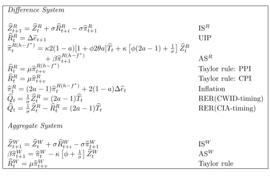
Table 1: Linearized system of equations
Difference System
b
ZR
t+1=ZbtR+σRbtR+i−σπbRt+1 ISR
b
RR
t = ∆bet+1 UIP
b
πR(h−f∗)
t =κ2(1−a)[1 +φ2θa]Tbt+κ
φ(2a−1) +σ1 bZR t
+βπbR(h−f∗)
t+1 ASR
b
RR t =µπb
R(h−f∗)
t+v Taylor rule: PPI
b
RR
t =µπbRt+v Taylor rule: CPI
b
πR
t = (2a−1)πb R(h−f∗)
t + 2(1−a)∆bet Inflation
b
Qt= 1σZbtR= (2a−1)Tbt RER(CWID-timing)
b
Qt= 1σZbtR−RbRt = (2a−1)Tbt RER(CIA-timing)
Aggregate System
b
ZW
t+1=ZbtW +σRbtW+i−σbπWt+1 ISW
βπbW
t+1=bπWt −κ
φ+σ1 bZW
t ASW
b
RW
t =µbπtW+v Taylor rule
Notes: The index R refers to the difference betweenhome and foreign variables e.g.
CtR ≡
Ct−
C∗t
,
πtR(h−f∗) ≡
πth−
π∗tf
. The index
W refers to world aggregates
whereπW =π+π∗
2 =
πh+π∗f
2 and ∆
et≡
et−
et−1.
trade changes will lead to different production responses in the two countries. For example,
a deterioration in theforeign terms of trade (Tbt↑) increases real marginal cost in theforeign
country (mcc∗
t ↑) and from theforeign equivalents to (29) and (31),foreign producer price
inflation (bπ∗f
t ↑) and output (Yb
∗
t ↑) both rise. From (40) a rise in foreign output, implies
a decrease in the real marginal cost ofhome producers which from (29) and (31) results in
a decline inhome producer price inflation (πbt↓) and output (Ybt↓). However ifσ > θ then home and foreign goods are complements and there is a positive spillover effect. Thus in
response to changes in the terms of trade,home (Ybt) andforeign (Ybt∗) output will expand
or contract together. Only in the special case of σ = θ are production spillover effects
absent.18
Since the two countries are symmetric, we employ the Aoki (1981) decomposition
ap-proach in order to analyze the determinacy properties of the model. The Aoki decomposition
decomposes the model into two decoupled dynamic systems: the aggregate system that
cap-18As discussed by Benigno and Benigno (2003) whenθ=σno spillover effects on production exist as the two
tures the properties of the closed world economy and the difference system that portrays the
open economy dimension. Thus, we solve both for cross-country differencesXR≡Xb−Xb∗
and worldwide aggregates19 XW ≡
X
2 +
X∗
2 . Determinacy of the aggregate and difference
systems implies determinacy at the individual country level since Xb = XW + XR
2 and
b
X∗
=XW −XR
2 . The complete linearized system of equations is summarized in Table 1.
2.7
Parameterization
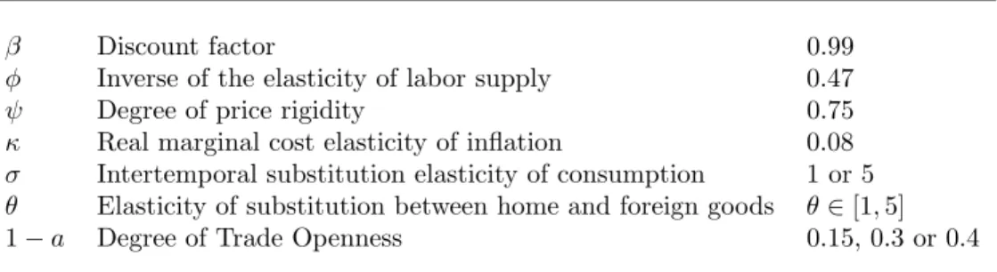
In order to illustrate the conditions for determinacy, the ensuing analysis uses the following
baseline parameter values summarized in Table 2. Parameterβis standard in the literature,
φis taken from Woodford (2003) and ψfrom Taylor (1999). Setting ψ= 0.75 constitutes
an average price duration of one year and this implies that the real marginal cost elasticity
of inflation κ = 0.08. Rotemberg and Woodford (1997) estimate σ = 6.37 for the US
economy. We follow Chari et al. (2002) and Llosa and Tuesta (2008) and initially set a
slightly lower value ofσ= 5. Settingσ= 5 implies a value of the risk aversion coefficient of
1/σ= 0.2. This value is lower than the range of estimates obtained from micro-level studies
(e.g. Vissing-Jorgensen (2002)) that typically suggest a risk aversion coefficient 1/σ ≥1.
Thus an alternative choice of σ = 1 is also examined.20 Empirical studies offer no clear
conclusion on the magnitude ofθ. Micro-level studies (e.g. Harrigan (1993)) suggest a value
of around 5 whereas macro-level studies (e.g. Bergin (2006)) suggest a much lower value of
around 1. Thus we compute the numerical eigenvalues of the model for alternative values
of θ∈[1,5]. Finally, three alternative values for the degree of trade openness (1−a) are
also chosen, which are roughly consistent with the ratio of imports to GDP of the USA
(a= 0.85), UK (a= 0.7) and Canada (a= 0.6).
19The determinacy conditions for the aggregate system are identical to comparable closed-economy New
Keynesian models (e.g. Carlstrom and Fuerst (2001)). Note the measure of inflation targeted is irrelevant in the aggregate system since producer and consumer price inflation are the same concept. i.e. πW =
π+π∗
2 =
πh+π∗f
2 .
20Woodford (2003) argues that a low risk aversion coefficient is justified on the grounds that the
Table 2: Baseline parameter values
β Discount factor 0.99
φ Inverse of the elasticity of labor supply 0.47
ψ Degree of price rigidity 0.75
κ Real marginal cost elasticity of inflation 0.08
σ Intertemporal substitution elasticity of consumption 1 or 5
θ Elasticity of substitution between home and foreign goods θ∈[1,5]
1−a Degree of Trade Openness 0.15, 0.3 or 0.4
3
Equilibrium Determinacy
This section considers the issue of local equilibrium determinacy. A key conclusion to
arise from the analysis is that the timing equivalence result does not generally hold for
open economies. As a consequence, whether monetary policy should react to producer price
inflation or consumer price inflation, in order to minimize policy-induced real indeterminacy,
crucially depends on the measure of money that enters into the utility function. The analysis
proceeds as follows. First, the breakdown of the timing equivalence result for open economies
is established by considering interest rate rules that react only to producer price inflation.
Here the conditions for equilibrium determinacy are examined when monetary policy is
characterized by a forward-looking interest rate rule under CWID-timing or a
current-looking rule under CIA-timing. After examining the indeterminacy implications of targeting
producer price inflation, the analysis then considers how the determinacy conditions differ
when monetary policy reacts to consumer price inflation under both timing assumptions.
3.1
Breakdown of the Timing Equivalence Result
Carlstrom and Fuerst (2001) show that for a standard New Keynesian closed-economy
model, the determinacy conditions for a forward-looking rule with CWID-timing is
analo-gous to the determinacy conditions for a current-looking rule with CIA-timing: i.e.
1< µ <1 + 2(1 +β)
This subsection shows the breakdown of this timing equivalence result for the open economy
under producer price inflation targeting.
Proposition 1 Suppose that monetary policy reacts to forward-looking (current-looking)
producer price inflation under CWID (CIA) timing. Then the necessary and sufficient
conditions for equilibrium determinacy are:
(a) Forward-looking rule (CWID-timing)
• Aggregate System / Closed Economy
1< µ <1 + 2(1 +β)
κ(1 +σφ)
• Difference System
1< µ <1 + 2(1 +β)
κ[1 +φσ+ 4φa(1−a)(θ−σ)]
• Open Economy
1< µ <1 + 2(1 +β)
κ(1 +σφ) if θ≤σ, or (42a)
1< µ <1 + 2(1 +β)
κ[1 +σφ+ 4φa(1−a)(θ−σ)] if θ > σ. (42b)
(b) Current-looking rule (CIA-timing)
• Aggregate System / Closed Economy
1< µ <1 + 2(1 +β)
κ(1 +σφ)
• Difference System
i. 2aθ≥σ(2a−1)and
µ >1 if 4a(1−a)φθ≥φσ(2a−1)(3−2a) + 1, or
1< µ < 2(1 +β) +κΛ1
ii. 2aθ < σ(2a−1)and
1< µ < 1−β
2κφ(1−a)[σ(2a−1)−2aθ] if 4a(1−a)φθ≥φσ(2a−1)(3−2a)+1, or
1< µ <min
2(1 +β) +κΛ
1
κ[1 +σφ(2a−1)(3−2a)−4a(1−a)φθ],
1−β
2κφ(1−a)[σ(2a−1)−2aθ]
if 4a(1−a)φθ < φσ(2a−1)(3−2a) + 1,
where Λ1≡1 +σφ+ 4aφ(1−a)(θ−σ).
• Open Economy
1< µ <1 + 2(1 +β)
κ(1 +σφ) if 2aθ≥σ(2a−1), or (43a)
1< µ <min
(1−β)
2κφ(1−a) [2a(σ−θ)−σ],1 +
2(1 +β)
κ(1 +σφ)
if 2aθ < σ(2a−1).
(43b)
Proof. See Appendix 5.1.
The following remark directly follows from Proposition 1.
Remark 1 (Timing Equivalence Result for Open Economies) The determinacy conditions
for a forward-looking rule under CWID-timing are analogous to a current-looking rule under
CIA-timing for the open economy, if and only if, θ=σ, i.e.
1< µ <1 + 2(1 +β)
κ(1 +σφ).
As summarized by Remark 1, the timing equivalence result holds for the open economy, if
and only if, the intertemporal substitution elasticity of consumption is equal to the elasticity
of substitution between home and foreign goods (σ = θ). In this case the determinacy
conditions for CWID and CIA-timing are analogous i.e. (42a) = (43a). As discussed
in Section 2.6, with σ = θ there are no international spillover effects in production as
the two countries are insular. Hence, this also explains why with σ=θ the determinacy
conditions for the open and closed economy are the same i.e. (41) = (42a) = (43a). However
if θ 6= σ then the timing equivalence result breaks down and the timing assumption on
indeterminacy.
First consider the case when the goods produced in the two countries are substitutes
(σ < θ) and thus there are negative spillover effects between the two countries. Inspection
of condition (42b) highlights that under CWID-timing the upper bound on the inflation
coefficient is reduced relative to (41) and this upper bound gets progressively smaller the
greater the difference betweenθ−σ >0 and the higher the degree of trade openness:
∂(42b)
∂a =
8(1 +β)κφ(θ−σ)(2a−1)
κ2[1 +σφ+ 4φa(1−a)(θ−σ)]2 >0 for any θ > σ. (44)
This is in stark contrast to CIA-timing where from (43a), if the goods are substitutes the
same upper bound on the inflation coefficient exists for both the open and closed-economy
i.e. (41) = (43a).
Now consider the case when the goods produced in the two countries are complements
σ > θ, thereby implying positive spillover effects between the two countries. Under
CWID-timing then from (42a) the determinacy conditions for the open and closed-economy
cor-respond exactly. However under CIA-timing, ifθ < σ(2a−1)
2a . inspection of condition (43b)
highlights that the potential range of indeterminacy is greater in the open economy provided
that (1−β)
2κφ(1−a)[2a(σ−θ)−σ] <1 +
2(1+β)
κ(1+σφ). If this is satisfied then:
∂(43b)
∂a =
2(1−β)κφ[4a(σ−θ)−σ] [2κφ(1−a) [2a(σ−θ)−σ]]2 ≷0
which implies that as the degree of trade openness increases, the potential range of
indeter-minacy increases if 4a(σ−θ)−σ >0 and decreases if 4a(σ−θ)−σ <0.
The results presented above suggest that Carlstrom and Fuerst’s (2001) observation that
a forward-looking rule with CWID-timing is equivalent to a current-looking rule with
CIA-timing does not typically hold in an open economy setting. The explanation for why this
timing equivalence breaks down in the open economy follows because the timing convention
adopted has no effect on the uncovered interest parity (UIP) condition (20). Intuitively
this can be most evidently seen by inspecting the linearized IS condition for the difference
system under each timing convention. The linearized IS equation for thehome country (28)
and itsforeignequivalent implyZbR
and CPI inflation differential (32) equations, the linearized IS conditions for the difference
system can be expressed as:
CWID: ZbtR+1=ZbtR+σ(2a−1)
b
RRt −bπ R(h−f∗)
t+1
(45)
CIA: ZbtR+1=ZbtR+σRbRt+1−σ(2a−1)πb R(h−f∗)
t+1 −2σ(1−a)RbRt. (46)
Note that under CIA-timing, the last term of (46) enters as a direct result of the UIP
condition. In a closed economy this last term disappears (i.e. a= 1) and sinceσ(2a−1)
becomesσ, the only difference in a closed economy between (45) and (46) is that the nominal
interest rate in the latter is scrolled forward one period. Thus the timing equivalence result
for a closed economy directly follows. However in the presence of international spillover
effects (σ6=θ), there can be no timing equivalence in the open economy without the interest
rate in the UIP term also being scrolled forward one period. Hence with the regular UIP
condition the timing equivalence of (45) and (46) breaks down since scrolling the interest
rate in the former no longer replicates the IS condition under CIA-timing.
3.2
CWID vs. CIA-timing: Indeterminacy Implications of
Target-ing Producer Price Inflation
Lets now illustrate the regions of indeterminacy using the baseline parameter values
sum-marized in Table 2 of Section 2.7 for policy rules that react to producer price inflation. As
discussed in the previous subsection, if there are negative (positive) international spillover
effects then there is more likely to be indeterminacy in an open economy compared to a
closed economy under CWID (CIA) timing. First, suppose that the policy rule reacts to
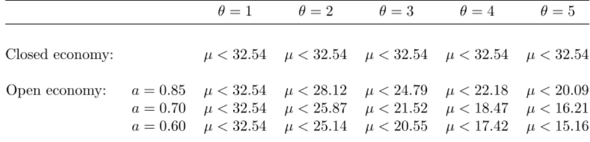
forward-looking producer price inflation under CWID-timing.21 Table 3 summarizes the
relevant upper bounds in the inflation response coefficient (µ) whenσ= 1.22 In accordance
with (44), the upper bounds computed for the open-economy decrease the higher isθ−σ >0
and the greater the degree of trade openness (lower isa). However, while these upper bounds
are considerably lower in the open economy relative to the closed economy for all cases of
σ < θ, they are still of a sizable magnitude to be deemed very unlikely to bind. Hence, for
21The determinacy conditions of this policy rule are given by (42a) and (42b) of Proposition 1.
22We do not report the case whenσ= 5 since that would require values ofθmuch greater than the empirical
Table 3: Upper bound computations on the inflation response coefficient (µ) for determinacy under CWID-timing (σ= 1)
θ= 1 θ= 2 θ= 3 θ= 4 θ= 5
Closed economy: µ <32.54 µ <32.54 µ <32.54 µ <32.54 µ <32.54
Open economy: a= 0.85 µ <32.54 µ <28.12 µ <24.79 µ <22.18 µ <20.09
a= 0.70 µ <32.54 µ <25.87 µ <21.52 µ <18.47 µ <16.21
a= 0.60 µ <32.54 µ <25.14 µ <20.55 µ <17.42 µ <15.16
both open and closed economies, a policy rule that targets future producer price inflation
under CWID-timing does not seem to matter for equilibrium determinacy at a practical
level.
Now suppose that the policy rule targets contemporaneous producer price inflation under
CIA-timing.23 In the presence of significant positive spillover effects between the two
coun-tries, such that 2aθ < σ(2a−1), then from (43b) of Proposition 1 the inflation coefficient
is constrained by two upper bounds: 1< µ <minΓ1,Γ2 where Γ1≡ (1−β)
2κφ(1−a)[2a(σ−θ)−σ]
and Γ2≡1 + 2(1+β)
κ(1+σφ). The second upper bound Γ2is identical to the determinacy
require-ments for a closed economy and this bound is unlikely to bind for reasonable parameter
values. For example, using the baseline parameter values outlined in Table 2 of Section 2.7,
ifσ= 5 then Γ2≈14.84. However, under the baseline parameterization the first bound Γ1
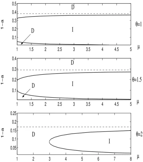
is much more likely to bind. Figure 1 depicts the regions in the parameter space (1−a,µ)
that are associated with determinacy (D) and indeterminacy (I) whenσ= 5 for three
alter-native values ofθ= 1,1.5,2. The dashed-lines in Figure 1 illustrate the value ofarequired
for 2aθ=σ(2a−1) and thus this upper bound Γ1ceases to apply.24 Figure 1 suggests that
the upper bound on the inflation coefficient µ given by Γ1 can be small. For example, if
θ= 1 then only for a very low degree of trade openness or a sufficiently high degree of trade
openness is Γ1unlikely to bind. However asθincreases the range of determinacy widens
sig-nificantly. Thus for values ofθ consistent with Bergin (2006) equilibrium indeterminacy is
a potential problem when the policy rule targets contemporaneous producer price inflation
under CIA-timing.25
23The determinacy conditions of this policy rule are given by (43a) and (43b) of Proposition 1. 24As shown by (43a) of proposition 1, determinacy in this case requires that 1< µ <Γ2.
1
1.5
2
2.5
3
3.5
4
4.5
5
0.1
0.2
0.3
0.4
0.5
µ
1−a
1
1.5
2
2.5
3
3.5
4
4.5
5
0.1
0.2
0.3
0.4
µ
1−a
1
2
3
4
5
6
7
8
0.05
0.1
0.15
0.2
0.25
µ
1−a
θ
=1
θ
=1.5
θ
=2
D
I
D
D
I
D
D
I
Figure 1: Regions of indeterminacy under a current-looking producer price inflation rule with CIA-timing (σ= 5)
The preceding analysis suggests that in the absence of a timing equivalence result for
open economies, the problem of indeterminacy increases under producer price inflation
targeting as we replace CWID-timing with CIA-timing. The explanation behind this finding
can be seen by comparing the Aggregate Supply (AS) condition implied by each timing
convention. Using equations (29), (30) and (31) and theirforeign equivalents, implies the
following linearized Aggregate Supply (AS) condition for the difference system: bπR(h−f∗)
t =
κ2(1−a)[1 +φ2θa]Tbt+κ
φ(2a−1) + 1
σ bZtR. Using (33) and the respective linearized
risk sharing conditions (35) and (36) to eliminate Tbt, the linearized AS equation for the
difference system can be expressed as:
CWID: πbR(h−f∗)
t = (κTζ+κZ)ZbtR+βbπ R(h−f∗)
CIA: πbR(h−f∗)
t = (κTζ+κZ)ZbtR+βbπ R(h−f∗)
t+1 −σκTζRbRt (48)
whereκT ≡2κ(1−a)[1 + 2aφθ]>0,κZ≡κ[φ(2a−1) + 1/σ]>0 andζ≡[σ(2a−1)]−1>0.
First note that in a closed economy the AS equations are the same under the two timing
conventions i.e. ifa= 1 then κT is zero and (47) and (48) collapse tobπR (h−f∗)
t =κZZbtR+
βbπR(h−f∗)
t+1 . However, for open economies, inspection of the above equations suggest that
the dynamics of producer price inflation crucially depends on the terms of trade, which
in turn depends on how money is introduced into the model. Under CWID-timing the
dynamics of the terms of trade are embed into the dynamics of the output gap since they
are proportional to one another from the RER condition: σ1ZbR
t = (2a−1)Tbt. In contrast
under CIA-timing the interest rate drives a wedge between the terms of trade and the
output gap since σ1ZbR
t −RbRt = (2a−1)Tbt. Thus under CIA-timing the nominal interest rate
also enters into the AS equation for open economies as a negative cost shock. Consequently
there are now two channels where the terms of trade affect producer price inflation and
these channels can yield opposite effects on the local dynamics of the economy. Given the
policy ruleRbR t =µbπ
R(h−f∗)
t then under CIA-timing, (48) can be alternatively expressed as
CIA: bπR(h−f∗)
t =
κ
Tζ+κZ
1 +µσκTζ
b
ZR t +
β
1 +µσκTζ
b
πR(h−f∗)
t+1 . (49)
By comparing the coefficients forZbR t andπb
R(h−f∗)
t+1 given in the AS equations (47) and (49),
a by-product of CIA-timing is that current domestic inflation (bπR(h−f∗)
t ) is less responsive
to changes in domestic demand and future domestic inflation.
3.3
Producer Price Inflation Targeting vs. Consumer Price
Infla-tion Targeting
A key question for monetary policy setting in open economies is whether producer price
inflation might be a better target than consumer price inflation. As this subsection shows,
in terms of equilibrium determinacy, whether the policy rule should react to producer or
3.3.1 Forward-Looking Rules Under CWID-timing
The criteria for determinacy when the monetary authority reacts to future consumer price
inflation is summarized in Proposition 2.
Proposition 2 Suppose that monetary policy reacts to forward-looking consumer price
in-flation under CWID timing. Then the necessary and sufficient conditions for equilibrium
determinacy are:
• Aggregate System / Closed Economy
1< µ <1 + 2(1 +β)
κ(1 +σφ) (50)
• Difference System
1< µ <min
1
2(1−a),
2(1 +β) +κΛ1
κΛ1+ 4(1 +β)(1−a)
• Open Economy
1< µ < 2(1 +β) +κΛ1 κΛ1+ 4(1 +β)(1−a)
(51)
whereΛ1≡1 +σφ+ 4φa(1−a)(θ−σ).
Proof. See Appendix 5.2.
Proposition 2 shows that the indeterminacy problem is more severe in open economies with
CWID-timing under a forward-looking consumer price inflation rule. This follows from
comparing the upper bound on the inflation response coefficient (µ) of condition (51) with
(50).26 The impact that the degree of trade openness has on the upper bound in condition
(51) is given by:
∂(51)
∂a =
4(1 +β) [κ[1 + 2φθ−φσ−4φ(θ−σ)a(1−a)] + 2(1 +β)] [κΛ1+ 4(1 +β)(1−a)]2
>0 (52)
and thus the greater the degree of trade openness, the higher the range of indeterminacy.
It is also important to note that the relative size of σ and θ have little significance for
26Is straightforward to verify that 2(1+β)+κΛ1
κΛ1+4(1+β)(1−a)<1 + 2(1+β)
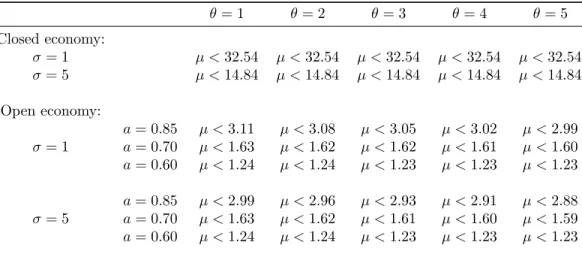
Table 4: Upper bound computations on the inflation response coefficient (µ) for determinacy under a forward-looking CPI rule with CWID-timing
θ= 1 θ= 2 θ= 3 θ= 4 θ= 5
Closed economy:
σ= 1 µ <32.54 µ <32.54 µ <32.54 µ <32.54 µ <32.54
σ= 5 µ <14.84 µ <14.84 µ <14.84 µ <14.84 µ <14.84
Open economy:
a= 0.85 µ <3.11 µ <3.08 µ <3.05 µ <3.02 µ <2.99
σ= 1 a= 0.70 µ <1.63 µ <1.62 µ <1.62 µ <1.61 µ <1.60
a= 0.60 µ <1.24 µ <1.24 µ <1.23 µ <1.23 µ <1.23
a= 0.85 µ <2.99 µ <2.96 µ <2.93 µ <2.91 µ <2.88
σ= 5 a= 0.70 µ <1.63 µ <1.62 µ <1.61 µ <1.60 µ <1.59
a= 0.60 µ <1.24 µ <1.24 µ <1.23 µ <1.23 µ <1.23
determinacy when the policy rule targets consumer price inflation, a stark contrast to when
the policy rule targets producer price inflation. For example, in the case when production
spillover effects are absent between the two countries (σ = θ), the upper bound given in
(51) collapses to
1< µ < 2(1 +β) +κ[1 +σφ] κ[1 +σφ] + 4(1 +β)(1−a).
Comparing this upper bound with (50) it is straightforward to see that determinacy is still
relatively lower in the open economy because of the presence of the degree of trade openness.
We illustrate the regions of indeterminacy using the baseline parameter values
sum-marized in Table 2 of Section 2.7. Table 4 summarizes the relevant upper bounds in the
inflation response coefficient (µ) for values of σ= 1 and σ= 5. In accordance with (52),
the upper bounds computed for the open-economy decrease the greater the degree of trade
openness (lower isa). For all combinations of θ and σ and for all values of a, the upper
bounds are not only considerably lower in the open economy relative to the closed economy,
but they are of an empirically relevant magnitude to suggest that equilibrium indeterminacy
could be a serious problem.
Comparing the determinacy condition (51) of Proposition 2 with conditions (42a) and
(42b) of Proposition 1, one clear conclusion to emerge under CWID-timing is that in terms
1 5 10 15 0.05
0.1 0.15 0.2 0.25 0.3 0.35
0.4 θ=1; σ=5
µ
1−a
1 5 10 15 20
0.05 0.1 0.15 0.2 0.25 0.3 0.35
0.4 θ=5; σ=1
µ
1−a
I
I
D D
Additional area of Indeterminacy under CPI targeting
Additional area of Indeterminacy under CPI targeting
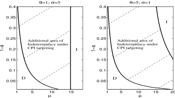
Figure 2: Regions of indeterminacy under forward-looking rules with CWID-timing
inflation.27 This conclusion can be easily illustrated for the baseline parameterization. For
these two alternative measures of inflation, Figure 2 depicts the regions in the parameter
space (a,µ) that are associated with determinacy (D) and indeterminacy (I) for two
alterna-tive combinations of (σ,θ). By inspection, reacting to consumer price inflation substantially
increases the range of indeterminacy. This finding coincides with the conclusion of the
ex-isting literature (e.g. Linnemann and Schabert (2006) and Llosa and Tuesta (2008)) and is
the basis for advocating that monetary policy should target producer price inflation, rather
than consumer price inflation, in order to minimize policy-induced indeterminacy for open
economies.
3.3.2 Current-Looking Rules Under CIA-timing
The criteria for determinacy when the monetary authority reacts to contemporaneous
con-sumer price inflation under CIA-timing is summarized in Proposition 3.
Proposition 3 Suppose that monetary policy reacts to current-looking consumer price
in-flation under CIA timing. Then the necessary and sufficient conditions for equilibrium
27By comparing the upper bounds on the inflation coefficient it is straightforward to show that this upper
bound is relatively lower under consumer price inflation targeting: i.e.κΛ1+4(1+2(1+β)+βκ)(1Λ1−a) <1 +κ2(1+(1+σφβ)) and
2(1+β)+κΛ1
κΛ1+4(1+β)(1−a) <1 +
2(1+β)
determinacy are:
• Aggregate System / Closed Economy
1< µ <1 + 2(1 +β)
κ(1 +σφ) (53)
• Difference System
(a) 4(1−a)(1 +β)≥κ[φσ+ 4a−3−4φa(1−a)(θ+σ)]:
µ >1 and either
(i)|a2|>3 or (ii) a02−a0a2+a1>1
(b) 4(1−a)(1 +β)< κ[φσ+ 4a−3−4φa(1−a)(θ+σ)]:
1< µ < 2(1 +β) +κΛ1
κ[φσ+ 4a−3−4φa(1−a)(θ+σ)]−4(1−a)(1 +β)
and either
(i)|a2|>3 or (ii) a02−a0a2+a1>1
whereΛ1≡1 +σφ+ 4aφ(1−a)(θ−σ).
• Open Economy
1< µ <1 + 2(1 +β)
κ(1 +σφ) (54a)
and either
(i)|a2|>3 or (ii) a20−a0a2+a1>1 (54b)
whereaj, j= 0,1,2 are given in Appendix5.3.
Proof. See Appendix 5.3.
If the policy rule reacts to contemporaneous consumer price inflation, then Proposition
3 shows that under CIA-timing the upper bound on the inflation coefficient is the same
for both closed and open economies i.e. (54a) = (53). Thus provided at least one of
economy mirror the closed economy. For the baseline parameter values summarized in Table
2 in Section 2.7 the numerical analysis suggests that condition (ii) of (54b) is always satisfied
for anyµ >1. Noting that this determinacy condition can be expressed as:
2(1−a)
β µ[2(1−a)µ(1−β) +κΛ1(µ−1)−κµ2(1−a)[1 + 2aθφ]−1]
+(1−β) + 2β(1−a)µ+κµ2(1−a)[1 + 2aθφ]>0,
then this becomes transparent by considering the case where β → 1 since this condition
collapses to:
µ+ 2aφθ+ (2a−1)φσ(µ−1)>0.
Therefore the determinacy properties of the closed and open economy are approximately
the same under CIA-timing if policy reacts to contemporaneous consumer price inflation.
However this is in stark contrast to producer price inflation targeting, where from the
analysis presented in Section 3.2, equilibrium indeterminacy is a potentially more serious
problem. Thus we can conclude that under CIA-timing, consumer price inflation is
prefer-able to producer price inflation in order to minimize policy-induced indeterminacy for open
economies.
3.3.3 Discussion
To summarize, the previous subsections showed that the preference towards a particular
inflation index, suggested by the criteria for equilibrium determinacy, crucially depends
upon the timing assumption on money employed. Under CWID-timing, it was shown that
producer price inflation is preferable in preventing equilibrium indeterminacy, whereas
un-der CIA-timing, targeting consumer price inflation is preferable. To decipher this result
intuitively, the key is to understand why the problem of indeterminacy is mitigated as we
replace CWID-timing with CIA-timing under consumer price inflation targeting.
Using the linearized equation for the CPI inflation differential (32) and the UIP condition
(34), the interest rate rule under CPI targeting for the difference system can be expressed
as:
b
RR
t =µ(2a−1)bπ R(h−f∗)
If the interest-rate rule is forward-looking (v = 1) then the reaction to future inflation
may be negative for highµand lowa. Hence monetary policy activeness against consumer
price inflation expectations and trade openness may provoke indeterminacy. However if the
interest rate rule is current-looking (v = 0) from (55) this generates policy inertia which
increases the likelihood of determinacy. This policy inertia appears as a result of the UIP
condition and is not present in the closed economy (i.e. a= 1).
The intuition for why under CIA-timing, contemporaneous consumer price inflation rules
exhibit policy inertia in the open economy, rests with how changes in the terms of trade
affect the dynamics of the CPI inflation rate. In an open economy thehome CPI inflation
rate depends on both the rate of producer price inflation and the terms of trade:
b
πt+v=bπth+v+ (1−a)
b
Tt+v−Tbt+v−1
(56)
where v = 1 under future inflation targeting and v = 0 under contemporaneous inflation
targeting. Under CWID-timing, the policy rule reacts to forward-looking consumer price
inflation (v= 1). Given that an increase in the real interest rate of thehomecountry results
in a current improvement in the terms of trade (Tbt↓), then in response to a non-fundamental
shock, inflationary expectations are self-fulfilling and indeterminacy is generated provided
b
πt+1 ↑. Whereas, indeterminacy depends on the sign of international spillover effects (i.e.
the relative size of σand θ) under producer price inflation targeting, as shown in (56) for
consumer price inflation targeting, indeterminacy depends on the relative weight of changes
in producer price inflation and adjustments in the terms of trade. For example, suppose that
an increase in the real interest rate, lowers real marginal cost putting downward pressure
on the producer price inflation rate πbh
t+1 ↓ and from (56) downward pressure on the CPI
inflation rate. With v = 1 the improvement in the terms of trade (Tbt ↓) associated with
an increase the real interest rate, from (56) generates upward pressure on the CPI inflation
rate. Since the degree of trade openness determines the influence of the terms of trade on
the CPI inflation rate, if this effect is strong enough, the CPI inflation rate can actually rise
despite producer price inflation falling, thus validating the initial inflationary belief.
Under CIA-timing the policy rule reacts to contemporaneous-looking consumer price
the terms if trade (Tbt↓) exerts downward pressure on CPI inflation. For example, suppose
that an increase in the real interest rate results in putting upward pressure on the producer
price inflation (which as discussed in Sections 3.1 and 3.2. requires positive international
spillover effects). With v = 0 the improvement in the terms of trade generates upward
pressure on the CPI inflation rate making indeterminacy less likely if the consumer price
inflation is targeted. In other words, monetary policy, through targeting contemporaneous
consumer price inflation, can help to prevent self-fulfilling inflation expectations by offsetting
the negative cost shock to producer price inflation introduced through CIA-timing.
4
Conclusion
In the design of monetary policy it is imperative that a proposed policy rule does not
introduce real indeterminacy and thus self-fulfilling fluctuations into the economy. For
open economies, a key policy question relates to which index of inflation central banks
should target in the policy rule. Recent research has advocated the targeting of producer
price inflation, since the targeting of consumer price inflation may lead to welfare-reducing
sunspot fluctuations. The contribution of this paper was to demonstrate that such policy
recommendations are highly sensitive to the timing of money employed in the determinacy
analysis.
This paper has shown that the timing equivalence result for a closed economy does
not generally apply for open economies due to the presence, in the latter, of international
spillover effects in production. A corollary of this is that different timing assumptions on
money, that have no consequences for equilibrium determinacy in a closed economy, can
have potentially non-trivial implications for indeterminacy in open economies. Using the
criteria for equilibrium determinacy, we have shown that the preferred index of inflation in
the policy rule is producer price inflation under CWID-timing, and consumer price inflation
under CIA-timing.
Consequently, in contrast with the existing literature, the results presented in this paper
suggest that on the grounds of equilibrium determinacy, central banks may be justified in