PreProcessing of MERIS, (A)ATSR and Vegetation Data for the ESACCI Project ‘FireDisturbance K.P. Günther, M. Habermeyer, M. Bachmann et al.
An Angular ThermalInfrared Data Acquisition System to Validate and Improve Satellite Products R. Niclòs, J.A. Valiente, M.A. Barberà et al.
Facilitate the Usage of Remote Sensing Surface Temperature on Surface Soil Moisture Estimation L. Zhuo & D. Han
Analysis of the Land Surface Temperature and NDVI Using MODIS Data on the Arctic Tundra During the Last Decade
C. Mattar, C. Durán-Alarcón, J. JiménezMuñoz & J.A. Sobrino
Climate OPT/IR
Validation of Simulated MM5Coupled PROMET Land Surface Temperatures Using MSG/SEVIRI Data B. Putzenlechner, F. Zabel, M. Muerth & W. Mauser
Implementation of EF from SEBS in a LUE Model in a Rapeseed Cropland N. Pardo, J. Timmermans, I.A. Pérez et al.
Monitoring Soil Infiltration in SemiArid Regions with Meteosat and a Coupled Model Approach Using PROMET and SLC
P. Klug, H. Bach & S. Migdall
The ESA STSE Changing Earth Science Network 20082013: Supporting the Next Generation of European Scientists
D. FernándezPrieto & R. Sabia
Bayesian Cloud Detection for Remote Sensing of Land Surface Temperature C.E. Bulgin, C. Old, C.J. Merchant et al.
Assessment of the Impact of ESA CCI Land Cover Information for Global Climate Model Simulations I.G. Khlystova, A. Loew, S. Hagemann et al.
Appropriate Treatment of Uncertainty and Ambiguity: A Flexible System for Climatological Calculations in Response to an On-Going Debate in the Transfer Velocity, K.
D.K. Woolf, L.M. GoddijnMurphy, J. Prytherch et al.
The Derivation of a CO2 Fugacity Climatology from SOCAT’s Global In Situ Data L.M. GoddijnMurphy, D.K. Woolf, P.E. Land & J.D. Shutler
Methods and Products OPT/IR
Automatic Selection of Training Areas Using Existing Land Cover Maps J. Silva, F. Bação, G. Foody & M. Caetano
Results from the Third Reprocessing of (A)ATSR Data S. O'Hara, P. Cocevar, H. Clarke & P. Goryl
Research and Applications with OPT/IR RS: Water
IMPLEMENTATION OF EF FROM SEBS IN A LUE MODEL IN A RAPESEED
CROPLAND
N. PARDO(1), J. TIMMERMANS(2), I. A. PÉREZ(1), M. A. GARCÍA(1), Z. SU(2), M. L. SÁNCHEZ(1)
(1)
Dept. of Applied Physics, University of Valladolid, Valladolid, Spain, Email: [email protected],
[email protected], [email protected], [email protected]
(2)
Dept. of Water Resources, Faculty of Geo–Information Science and Earth Observation (ITC), University of Twente, Enschede, The Netherlands, Email: [email protected], [email protected]
ABSTRACT
In assessment of global carbon cycle, evaluation of
gross primary production, GPP, of an ecosystem is the
main endeavour. The most adequate way to address
this study is to apply a Light Use Efficiency, LUE,
model in combination with an Eddy Covariance, EC,
system.
In this paper, evaporative fraction, EF, from two
different databases (ground-based measurements and
calculated by the Surface Energy Balance System,
SEBS, algorithm developed at ITC) are applied to a
LUE model in order to calculate a final value which
is the maximum PAR conversion efficiency of the
cropland.
The LUE model was found to fit properly using both
EF databases, with squared correlation coefficients of
0.89 and 0.81 for ground measurements and SEBS
results, respectively. Final values for maximum
efficiency were of 2.82 0.19 gC MJ-1 (measured EF)
and 2.59 0.23 gC MJ-1 (SEBS). All these results were
obtained with FPAR provided by MERIS.
1. INTRODUCTION
Longer temporal series of atmospheric CO2
concentration have been measured and recorded at
Mauna Loa observatory (http://www.cmdl.noaa.gov)
showing a continuous increasing trend. At present there
is general consensus regarding the influence of GHG
(greenhouse gases) on climate change. Increases in
surface temperature and sea level are clear indicators of
this change [1]. Changes in temperature together with
changes in the precipitation pattern can lead to a
stomatal closure, which influence the amount of CO2
sequestered by the ecosystem [2]. This fact can turn an
ecosystem from sink to source of carbon. Therefore,
knowledge of the behaviour of the different ecosystems
is an actual issue widely studied.
Regarding to climate change, assessment of the total
amount of CO2 assimilated by crops, GPP, and Net
Ecosystem Exchange, NEE, is a main challenge.
Measurements of these variables are usually made
using micrometeorological techniques such as EC.
Different biomes have been evaluated by installing EC
towers, and several networks have been established
around the world such as CARBOEUROFLUX,
ASIAFLUX or FLUXNET [3]. These networks
provide information of these studies, quantifying GPP
and NEE for different ecosystems and showing their
behaviour as sink or source of carbon. The results
obtained evidence the unequal ability to uptake CO2 in
different ecosystems [4].
An alternative for estimating GPP is based on the
application of LUE models [5, 6]. In these models EF
is used as an important parameter reducing final
value since low EF values are usually associated to
water stress.
In this study, in order to quantify the crop ability as a
CO2 sink, continuous measurements of NEE, latent and
sensible heat, LE and H, were made using an EC
station. Moreover, a LUE model has been calibrated
for a rapeseed crop using MERIS products, EF and
meteorological data. EF has been calculated using two
separately procedures. Firstly, ground measurements of
_____________________________________
LE and H were used. Secondly, EF results from SEBS
algorithm were employed.
This paper presents the results of the GPP 8–d
estimated values using a LUE model over a rapeseed
crop for the agricultural year using FPAR from
MERIS, and calculates the value characterizing the
studied rapeseed cropland.
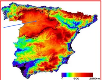
Figure 1. Location of the measuring plot
2. SITE DESCRIPTION
Measurements have been conducted continuously since
2008 in a farmland located about 30 km far from
Valladolid in the upper Spanish plateau (Fig. 1). Relief
elements are not present and horizontal homogeneity is
ensured. This is a required feature when
micrometeorological techniques are used to measure
ecosystem exchanges. The dominant land use is non–
irrigated crops with a rotating scheme including
rapeseed, wheat/barley, green peas, rye and sunflower.
During the studied period, rapeseed was grown.
Rapeseed was sown in September, 2007 and harvested
in July, 2008. Measurements started in March–April,
2008. First stages of the crop development were thus
missed. However, the period for which the crop
presented its full development (April–June), as well as
the senescence stages, was covered.
3. METHODOLOGY
3.1 MERIS data
MERIS images were downloaded from the MERCI
interface and processed with BEAM VISAT software
(version 4.8). The algorithm employed to retrieve
biophysical parameters was TOC (Top of Canopy)
Vegetation Processor. Detailed information concerning
the algorithm can be found in the literature [7, 8].
Values retrieved for LAI and FPAR corresponded to
the pixel centred on the measuring plot. Isolated gaps
were refilled by linear interpolation between the
previous and subsequent data or with the average value
calculated for pixels surrounding this central pixel.
MERIS images have a temporal resolution of
approximately 3 days and they have been used in
Reduced Resolution, RR, covering 1040 m x 1160 m.
Biophysical parameters retrieved from the sensor were
aggregated into 8–d composites for later calculations.
3.2 Field data
NEE, LE and H were measured using
micrometeorological instrumentation by applying the
EC technique. This instrumentation consists of an
IRGA (InfraRed Gas Analyzer, Li–7500) and a sonic
anemometer (USA–1) sampling at a frequency of
10Hz. Instantaneous data were processed each 30min.
TK2 software [9] was used to process these 30min
averages to ensure the quality of the turbulent fluxes
and ecosystem exchanges (water and carbon). The LUE
model applied needs of other ancillary data,
particularly meteorological measurements. The
meteorological instrumentation is placed in a tower
located a few meters from the tower housing the
micrometeorological instrumentation. This is equipped,
Photosynthetically Active Radiation, PAR, and sensors
measuring soil and air temperature and moisture. All
ground data were aggregated into 8–d composites in
the same way than MERIS biophysical parameters.
EF was calculated from LE and H measurements as
follows:
(1)
GPP, a fundamental parameter to calibrate the LUE
model, is indirectly derived by EC measurements as the
difference between ecosystem respiration, RE, and
NEE as follows:
(2)
CO2 total exchange plays a crucial role in the carbon
balance, particularly to define the ecosystem behaviour
as sink or source of carbon. Therefore, NEE and GPP
datasets must be gap-filled in order to quantify the
amount of carbon exchanged between the ecosystem
and the atmosphere.
RE can be measured experimentally using soil
chambers [10] or parameterized from meteorological
data. In this study, RE has been parameterized using
the soil moisture, SM, and the air temperature, T.
Since photosynthesis only takes place during daytime,
GPP takes thus value 0 during nighttime. Hence, RE
was determined using the NEE nocturnal data by
means of a parameterization using a modified Van’t
Hoff equation as follows:
· · exp · (3)
where the parameters a and b were obtained by a non–
linear fit using the Marquardt algorithm. Diurnal RE
was then computed using the fitted Eq. 3 together with
daytime values of SM and T.
In this paper, NEE gaps during daytime have been
filled by fitting a Michaelis–Menten equation relating
NEE and PAR [11],
· ·
· (4)
where is the apparent quantum yield, is the
maximum photosynthetic assimilation, and is the
ecosystem respiration. This equation was fitted for
each 15–days period in order to obtain the best results
regarding to changes in the crop development.
3.3 SEBS methodology
The single–source SEBS model [12] uses remote
sensing products to calculate all energy balance
components and EF.
Net radiation, RN, is calculated as the sum of short and
long–wave net radiation by applying the equations:
(5)
1 · (6)
· · · (7)
where and emis are the albedo and emissivity,
respectively, LST is the land surface temperature,
is the Stefan–Boltzmann constant, and and
are downward short and long–wave radiation,
respectively. Soil heat flux, G, is calculated from RN
using a non–linear equation [13]:
· · exp · (8)
where C and are fitted parameters.
H is calculated iteratively until the lowest error is
constrained between H values in dry and wet limits,
and .
Finally, EF is calculated using relative evaporation,
relevap, and H in the wet limit as follows:
· (9)
In this paper, the SEBS algorithm has been modified in
order to obtain better results for H and EF.
Modification has been applied to the calculation of the
roughness for heat transfer, zoh, used in H calculation
given by
(10)
where is the roughness height for momentum
transfer and kB-1 is a parameter depending on
biophysical parameters related to vegetation
development retrieved from remote sensing. A scale
factor depending on SM has been applied to the
calculation of kB-1 as described in the literature [14]. A
rescaled kB-1 parameter is obtained by applying this
scale factor, improving results for H and EF.
SM used in the scale factor is retrieved from the
AMSR–E sensor onboard Aqua satellite.
Further information concerning the SEBS algorithm
[12] and its modification [14] can be found in the
literature.
4. LUE MODEL
The LUE model proposed by Monteith is based on the
linear relationship between GPP and APAR, where
APAR is the product of direct ground PAR
measurements and FPAR provided by MERIS.
Different LUE models have been formulated taking
into account different vegetation indices [15]. In these
models the value for the efficiency has been usually
considered constant regardless of the ecosystem
studied [6, 15]. However, due to the wide influence of
the vegetation features in the efficiency, varies
greatly as a function of vegetation types, as well as
climate conditions.
Previous researches have evaluated how the lack of
water and changes in temperature limit the
photosynthetic activity of the vegetation [15, 16]. The
decrease in the photosynthetic activity and, therefore,
changes in the efficiency of the vegetation/ecosystem
due to water and temperature stress, are taking into
account using a scalar factor varying between 0 and 1.
In the model applied in this study temperature stress is
dependent on T and water stress is assumed to be equal
to EF [16, 17]. Therefore,
· · · · (11)
where is the maximum PAR conversion efficiency.
Eq. 11 can be reformulated as
· / (12)
where the subscript MERIS or SEBS indicates if EF
from ground or SEBS has been used, respectively, in
Eq. 11.
5. RESULTS
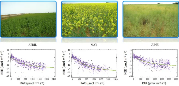
Relationship between NEE and PAR is shown in Fig. 2
and also the fit line obtained by applying Eq. 4. As an
example, months from April to June are displayed,
although in this study all available data for the whole
agricultural year are considered. For these months the
crop is fully developed and NEE presents its maximum
negative values. From this result can be inferred the
marked seasonal evolution of NEE and the crop
behavior as a CO2 sink (negative values of NEE),
Figure 2. Seasonal evolution of NEE (lower) and crop development (upper)
Maximum peak for CO2 uptake is found out in May
coinciding with the total development of the rapeseed
(see picture for May in Fig. 2). In June the crop starts
its senescence period and NEE reaches less negative
values than in previous months but still behaves as a
sink. GPP applied to the LUE model is calculated from
these direct measurements of NEE and respiration by
Eq. 2, once NEE and RE datasets have been gap-filled
using Eq. 3-4.
Since SM retrieved from AMSR–E is used by SEBS, a
comparative analysis between those values and
ground–measurements is made. Fig. 3 shows the
seasonal course followed for both datasets. As derived
from this graph, a similar pattern and good agreement
(slope = 0.55; R2 = 0.49) are found. This result probes
that SM retrieved from AMSR–E might be
representative for the studied plot in spite of the high
spatial resolution of AMSR–E (25km).
As stated before, the LUE model uses EF as a factor
to take into account water stress into the vegetation.
DATE
01Mar 01May 01Jul 01Sep 01Nov
S
o
il M
o
is
tu
re
(
%
)
0 10 20 30 40 50 60 70
SM_AMSRE SM_experimental
Figure 3. Comparison of the SM retrieved from
AMSRE and measured in the studied plot
In this paper, this parameter has been calculated using
two different approaches. So, two different EF datasets
have been obtained. Firstly, EF has been calculated
from ground measurements using Eq. 1. Separately, EF
has been determined by applying the SEBS model to
the studied plot. The comparison of both datasets,
depicted in Fig. 4, shows the similarities in the seasonal
that EF retrieved from SEBS tended to overestimating
the ground values during the whole year and
particularly after July (after the harvest). In summer,
EF values was expected to be lower due to the lack of
precipitation and vegetation cover. However, EF
retrieved from SEBS yielded unrealistic high values,
above 0.4 during this period and even higher in
autumn.
DATE
01Mar 01May 01Jul 01Sep 01Nov
EF 0.0 0.2 0.4 0.6 0.8 1.0 EF_experimental EF_SEBS
Figure 4. Comparative of the EF calculated from
ground measurements and SEBS–retrieved
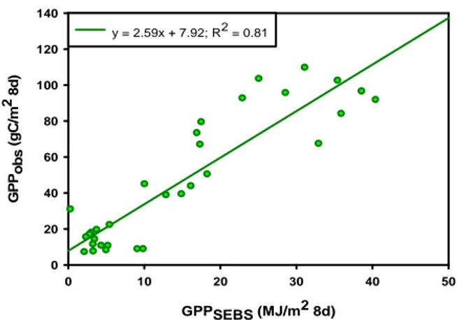
Finally, is inferred through the slope of the linear
regression fit given by Eq. 12. GPP observed (GPPobs)
is plotted against the GPP modelled (GPPMERIS/SEBS) as
shown in Figs. 5-6, and the goodness of the fit can be
derived. Estimated for the rapeseed, given by the
slope value, is 2.82 gC MJ-1 when EF used in the LUE
model is that obtained from ground measurements, and
2.59 gC MJ-1 when EF retrieved from SEBS is used.
The LUE model fitted properly the GPP estimates
using the EF from ground–measurements and that
calculated with SEBS with squared correlation
coefficient, , of 0.89 and 0.81, respectively.
values, independently the source of which EF is
retrieved, are slightly higher than other results reported
in the literature for crops [11]. The lower value
obtained when EF from SEBS is used might be
attributed to the high EF values during summer, which
does not seem to reflect the real lack of water for that
period.
GPPSEBS (MJ/m2 8d)
0 10 20 30 40 50
GP
Pobs
(g
C
/m
2 8d
) 0 20 40 60 80 100 120 140
y = 2.59x + 7.92; R2 = 0.81
Figure 5. LUE model applying the EF calculated with
SEBS model and MERIS data
GPPMERIS (MJ/m2 8d)
0 10 20 30 40 50
GP
Pobs
(g
C
/m
2 8d
) 0 20 40 60 80 100 120 140
y = 2.82 x + 10.49 ; R2 = 0.89
Figure 6. LUE model applying EF calculated from
ground measurements and MERIS data
6. CONCLUSIONS
A LUE model based on FPAR measurements retrieved
from MERIS and EF has been calibrated over a
rapeseed cropland in order to calculate the maximum
PAR conversion efficiency of this crop.
Water stress is taken into account in the LUE model
the rest of the parameters in Eq. 11 have been not
modified. Firstly, EF was calculated from ground
measurements of LE and H. Secondly, an energy
balance model (SEBS) was applied over the studied
plot to obtain a new EF dataset. A good agreement has
been found between both datasets; however, SEBS
tends to overestimate EF values. This overestimation is
more marked after the crop is harvested.
The SEBS model applied to calculate EF has been
modified by applying a scale factor dependent on SM.
An assessment of the SM used by the algorithm has
been made and a comparison between these values and
those measured is shown in this paper. Similar seasonal
pattern is found for the two SM datasets. These results
lead to consider SM values retrieved from AMSR–E
representative for the studied plot.
Finally, is calculated through the calibration of a
LUE model over a rapeseed crop. This parameter
presents lower differences whether the ground–based
or SEBS–based EF is used in the LUE model. Final
value obtained is slightly higher than the typical values
reported in the literature for crops. Besides, it should be
mentioned that the rapeseed has not been widely
studied and values for the efficiency of this crop are
rarely found in the literature. The high efficiency
values found in this study evidence the ability of the
rapeseed to behave as a CO2 sink.
7. ACKNOWLEDGEMENTS
This research has been conducted in the framework of
project CGL2009–11979 (MICINN) and funded
together with ERDF (The European Regional
Development Fund) funds. Authors wish to thank the
ESA for providing us the remote sensing images from
MERIS sensor used in this research. Authors express
also their gratitude to Carlos Blanco, for his
contribution to data processing, and Jerónimo Alonso,
owner of the Monte de Rocío farm where
measurements were carried out.
8. REFERENCES
1. IPCC. (2007). Climate Change 2007: The
Physical Science Basis. Contribution of Working
Group I to the Fourth Assessment Report of the
Intergovernmental Panel on Climate Change
[Solomon, S., Qin, D., Manning, M., Chen, Z.,
Marquis, M., Averyt, K.B., Tignor, M. & Miller,
H.L. (eds.)]. Cambridge University Press,
Cambridge, United Kingdom and New York, NY,
USA, 996 pp.
2. Meyers, T. P. (2001). A comparison of
summertime water and CO2 fluxes over rangeland
for well watered and drought conditions. Agric.
For. Meteorol. 106 (3), 205-214.
3. Baldocchi, D., Falge, E., Gu, L., Olson, R.,
Hollinger, D., Running, S., Anthoni, P.,
Bernhofer, C., Davis, K., Evans, R., Fuentes, J.,
Goldstein, A., Katul, G., Law, B., Lee, X., Malhi,
Y., Meyers, T., Munger, W., Oechel, W., Paw, U.
K. T., Pilegaard, K., Schmid, H. P., Valentini, R.,
Verma, S., Vesala, T., Wilson, K. & Wofsy, S.
(2001). FLUXNET: A new tool to study the
temporal and spatial variability of
ecosystem-scale carbon dioxide, water vapor, and energy
flux densities. Bull. Am. Meteorol. Soc. 82(11),
2415-2434.
4. Running, S. W., D. D. Baldocchi, D. P. Turner, S.
T. Gower, P. S. Bakwin, & K. A. Hibbard.
(1999). A global terrestrial monitoring network
integrating tower fluxes, flask sampling,
ecosystem modeling and EOS satellite data.
Remote Sens. Environ. 70 (1), 108-127.
5. Turner, D. P., Ritts, W. D., Cohen, W. B., Gower,
S. T., Zhao, M., Running, S. W., Wofsy, S. C.,
Urbanski, S., Dunn, A. L. & Munger, J. W.
over boreal and deciduous forest landscapes in
support of MODIS GPP product validation.
Remote Sens. Environ. 88(3), 256-270.
6. Sjöström, M., Ardö, J., Eklundh, L., El-Tahir, B.
A., El-Khidir, H. A. M., Hellström, M., Pilesjö, P.
& Seaquist, J. (2009). Evaluation of satellite
based indices for gross primary production
estimates in a sparse savanna in the Sudan.
Biogeosciences. 6(1), 129-138.
7. Gobron, N., B. Pinty, O. Aussedat, M. Taberner,
O. Faber, F. Mélin, T. Lavergne, M. Robustelli, &
P. Snoeij. (2008). Uncertainty estimates for the
FAPAR operational products derived from
MERIS - impact of top-of-atmosphere radiance
uncertainties and validation with field
data. Remote Sens. Environ. 112(4), 1871-1883.
8. Bacour, C., Baret, F., Béal, D., Weiss, M., &
Pavageau, K. (2006). Neural network estimation
of LAI, fAPAR, fCover and LAI×Cab, from top
of canopy MERIS reflectance data: principles and
validation. Remote Sens. Environ. 105(4),
313-325.
9. Mauder, M. & Foken, T. (2004). Documentation
and instruction manual of the eddy covariance
software package TK2. Arbeitsergebnisse,
Universität Bayreuth, Abt. Mikrometeorologie,
Print, ISSN 1614-8916.
10. Sánchez, M. L., Ozores, M. I., López, M. J.,
Colle, R., De Torre, B., García, M. A., & Pérez, I.
(2003). Soil CO2 fluxes beneath barley on the
central Spanish plateau. Agric. For.
Meteorol. 118(1-2), 85-95.
11. Wang, X., Ma, M., Huang, G., Veroustraete, F.,
Zhang, Z., Song, Y. & Tan, J. (2012). Vegetation
primary production estimation at maize and alpine
meadow over the Heihe River Basin, China. Int. J.
Appl. Earth Obs. Geoinf. 17 (1), 94-101.
12. Su, Z. The surface energy balance system (SEBS)
for estimation of turbulent heat fluxes. (2002).
Hydro. Earth Syst. Sci. 6(1), 85-99.
13. Kustas, W. P., Daughtry, C. S. T. & Van Oevelen,
P. J. (1993). Analytical treatment of the
relationships between soil heat flux/net radiation
ratio and vegetation indices. Remote Sens.
Environ. 46(3), 319-330.
14. Gokmen, M., Vekerdy, Z., Verhoef, A., Verhoef,
W., Batelaan, O. & van der Tol, C. (2012).
Integration of soil moisture in SEBS for
improving evapotranspiration estimation under
water stress conditions. Remote Sens. Environ.
121, 261-274.
15. Running, S. W., Thornton, P. E., Nemani, R. R.,
& Glassy, J. M. (2000). Global terrestrial gross
and net primary productivity from the earth
observing system. In O. Sala, R. Jackson, & H.
Mooney (Eds.), Methods in ecosystem science
(pp. 44 – 57). New York, Springer-Verlag
16. Yuan, W., Liu, S., Zhou, G., Zhou, G., Tieszen,
L. L., Baldocchi, D., Bernhofer, C., Gholz, H.,
Goldstein, A. H., Goulden, M. L., Hollinger, D.
Y., Hu, Y., Law, B. E., Stoy, P. C., Vesala, T. &
Wofsy, S. C. (2007). Deriving a light use
efficiency model from eddy covariance flux data
for predicting daily gross primary production
across biomes. Agric. For. Meteorol. 143(3-4),
189-207.
17. Xiao, X., D. Hollinger, J. Aber, M. Goltz, E. A.
Davidson, Q. Zhang & B. Moore III. (2004).
Satellite-Based modeling of gross primary
production in an evergreen needleleaf