Evaluating Connectivity and Quality in Ad-Hoc Networks through Clustering and Trellis Algorithms-Edición Única

Evaluating Connectivity and Quality in Ad-Hoc Networks

through Clustering and Trellis Algorithms-Edición Única

Title Evaluating Connectivity and Quality in Ad-Hoc Networks through Clustering and Trellis Algorithms-Edición Única Authors Martha Lucia Torres Lozano

Affiliation ITESM Issue Date 2003-05-01 Item type Tesis

Rights Open Access

Downloaded 19-Jan-2017 07:15:49

Instituto Tecnológico y de Estudios Superiores de

Monterrey

Campus Monterrey

División de Electrónica, Computación, Información, y

Comunicaciones

Programa de Graduados

Evaluating Connectivity and Quality in Ad-Hoc Networks

through Clustering and Trellis Algorithms

THESIS

Presented as a partial fulfillment of the requeriments for the degree of

Master of Science in Electronic Engineering

Major in Telecommunications

Martha Lucia Torres Lozano

Acknowledgments

I thank Instituto Tecnológico y de Estudios Superiores de Monterrey for the facilities pro-vicled. I am grateful to my thesis advisor, César Vargas Rosales, Ph.D., because this thesis could riot have been possible without his interest and collaboration. I mention specially to José Ramón Rodriguez Cruz, Ph,D., and Artemio Aguilar Coutiño, M.Sc., for their corriments that have helped to enhance this work.

My friends, Catalina, Beatriz, Carolina, Ericka, Franklin, Juan D., Fernando, Perla, Rafael and all my friends and partners from Colombia, México and CET for their friendship and helping in this period of time.

MARTHA LUCIA TORRES LOZANO

To my parents, Federico and Julia To my siblings, Diana and Lina

To my boyfriend, Eric

Evaluating Connectivity and Quality in Ad­Hoc Networks

through Clustering and Trellis Algorithms

Martha Lucia Torres Lozano, M.Sc.

Instituto Tecnológico y de Estudios Superiores de Monterrey, 2003

Abstract

Recently, wireless networks have becorne increasingly popular in the coinputing iridustry. These networks provide mobile users with ubiquitous coinputing capability and informa-tion access regardless of the locainforma-tion. There are currently two variainforma-tions of mobile wire-less networks- infrastructured (e.g., cellular network) and "infrastructurewire-less" networks, called Mobile Ad-Hoc Networks, where the entire network is mobile, and the individual termináis are allowed to move at will, relative to each other, theri they are self-creating, self-organizing, ancl self-aclmiriisteririg.

Contents

List of Figures iü

List of Tables v

Chapter 1 Introduction 1

1.1 Objective 2 1.2 Justification 2 1.3 Contribution 3 1.4 Organization 3

Chapter 2 Wireless Ad­Hoc Networks 5

2.1 Important Aspects about Ad-Hoc Networks 6 2.1.1 Traffic Profiles 6 2.1.2 Types of Ad-Hoc Networks 7 2.1.3 Security and Privacy 7 2.2 Characteristics of MANETs 7 2.3 Routing in Ad-Hoc Networks 8 2.4 Ad-hoc Mobile Routing Protocols 10 2.4.1 Table-Driven Approaches 11 2.4.2 Source-Initiated On-Demand Approaches 14 2.5 Quality of Service (QoS) 17

Chapter 3 Clustering in Ad­Hoc Networks 19

3.1 Clustering Algorithm 20 3.1.1 DMAC Algorithm 20 3.1.2 ABCP Algorithm 21 3.1.3 Application of the clustering algorithms to the sample scenario . . . 23 3.2 DDCA Algorithm 26 3.2.1 (cM) Cluster Framework 27

ii CONTENTS

3.2.3 Clustering Algorithm 29 3.3 Trellis Algorithm for Ad-Hoc Networks 33 3.3.1 Graph Modeling 33 3.3.2 Link and Path Cost 35 3.3.3 Algorithm Net to Trellis 36 3.3.4 Exarnple applying Trellis Algorithm 39 3.4 Connectivity and Quality of Network 47

Chapter 4 Model Description 49

4.1 Network Generation 49 4.2 Connectivity and Quality Application 51

Chapter 5 Numerical Results 57

5.1 Network Generation 57 5.1.1 Cluster Generation 57 5.1.2 Link Generation 57 5.2 Proposed Scenarios 59 5.2.1 Sceriario 1 59 5.2.2 Scenario 2 62 5.2.3 Scenario 3 71 5.2.4 Scenario 4 77

Chapter 6 Conclusión and Further Research 85

6.1 Conclusions 85 6.2 Further Research 87

Bibliography 89

List of Figures

2.1 Example of a simple Ad-Hoc Network with three participating nodes ... 6 2.2 Block Diagram of a mobile node acting both as hosts and as router . . . . 6 2.3 Ari Ad-Hoc Network example 8 2.4 Schemes for routing in Ad-Hoc Networks 9 2.5 Categorization of Ad-Hoc Routing Protocols 11 2.6 A CSGR path 12 2.7 Routing Inefficiericy in CGSR 13 2.8 ZRP and Concept of Bordercasting 16

3.1 Example of cluster of Ad-Hoc network 20 3.2 DCMA Flowchart 22 3.3 ABCP Flowchart 23 3.4 Initial Ad hoc Network 24 3.5 a) New Node, DMAC Algorithm. b)New Node, ABCP Algorithm 25 3.6 a) Link Failure, DMAC Algorithm. b)Link Failure, ABCP Algorithm. ... 25 3.7 a) New Link, DMAC Algorithm. b) New Link, ABCP Algorithm 26 3.8 General flowchart for DDCA Algorithm 27 3.9 Notation to Definition 1 29 3.10 Node Activation Flowchart 31 3.11 Link Activation Flowchart 32 3.12 Link Failure and Node Deactivation 34

3.13 A /C-Trellis graph with L=5, H=4 35

3.14 Illustration of application of the Operation Pl and P2 38 3.15 Trellis Algorithm Flowchart 39 3.16 Transformation frorn normal network to Trellis Graph 40 3.17 Initial Ad-Hoc Network 41 3.18 Applying the Trellis Algorithm in Cluster A 41 3.19 Trellis Algorithm applied to cluster B 42 3.20 Trellis Algorithm applied into cluster C 42

iv LIST OF FIGURES

3.21 Trellis Algorithm applied taking clusters as a noeles 42 3.22 Trellis Algorithm applied in all tlie network 43 3.23 Paths with minor probabilities 44 3.24 Link Failure Scenario 45 3.25 New Node Scenario 46 3.26 New link Scenario 46 3.27 Connectivity example 47 3.28 a) High Density of nodes, b) Low density of Nodes 48 4.1 Illustration of nodes, distances and Pr¿j of (4.3) 51 4.2 Network Generation Algorithm 52 4.3 Types of Connectivity at the network generated 52 4.4 Types of Quality at the network generated 54 5.1 Organization área in different nurnbers of cluster 58 5.2 Network Connected with 4 Clusters 58 5.3 Initial Network 60 5.4 Situations Scenario 1 61 5.5 Performance irito the Cluster(4 Clusters) 63 5.6 Performance into the Cluster (9 Clusters) 64 5.7 Performance into the Cluster (16 Clusters) 65 5.8 Total Cluster Performance for 100 nodes 66 5.9 Total Cluster Performance for 200 nodes 67 5.10 Total Cluster Performance for 400 nodes 67

5.11 TotalCBL and TotalQBL for 100 nodes 68

5.12 TotalCBL and TotalQBL for 200 nodes 69

5.13 TotalCBL and TotalQBL for 400 nodes 70

List of Tables

Chapter 1

Introduction

Since their emergence iri 1970's, wireless networks have become increasingly popular in the computing industry. These networks provide mobile users with ubiquitous computing capa-bility and information access regardless of the location. There are currently two variatioris of mobile wireless networks- infrastructured and "infrastructureless" networks.

The infrastructured networks (e.g., cellular network), have fixed, wired gateways and centralized administration for their operations. They have fixed base stations which are interconnected to other base stations. The transmission range of a base station constitutes a cell. All the mobile nodes lying within this cell connect to and communicate with the nearest bridge (base station), [1]. In contrast, infrastructureless networks, called Mobile Ad-Hoc Networks (MANET), do not have fixed routers. All nodes are capable of movement and can be connected dynamically in an arbitrary manner. The responsibilities for organizing and controlling the network are distributed among the termináis themselves, in other words, Ad Hoc wireless networks are self-creating, self-organizing, and self-adrninistering. The entire network is mobile, and the individual termináis are allowed to move at will, relative to each other. The nodes for this class of network can be located in or on airplanes, ships, trucks, cars, perhaps even on people or very small devices like laptops.

Communication, between arbitrary endpoints in ad hoc networks, requires routing over múltiple hops wireless-hop paths. The main difficulty arises because without a fixed infrastructure, these paths consist of wireless links whose endpoints are likely to be moving independently of one another. Consequently, node mobility causes the frequent failure and activation of links which leads to increased network congestión, while the network's routing algorithm reacts to the topology changes.

Unlike fixed infrastructure networks where link failures are comparatively rare events, the rate of link failure due to node mobility is the primary obstacle to routing in Ad-hoc networks. One possible solution for this problem, minimization of reaction to mobility, is to use a protocol based on a clustering system, this is the objective of this work, as well as to evalúate its advantages in terrns of network performance measures. A protocol is a set

2 CHAPTER 1. INTRODUCTION

of rules that governs the Communications between nodes in a network. These rules include guidelines that regúlate the following characteristics of a network: access method, allowed physical topologies, types of cabling, and speed of data transfer. A cluster is a group of similar things (e.g., nodes in telecommunications systems), with similar characteristics. Then, protocols based on a clustering system consist of a set of rules applying cluster partition, where noeles have autonomously organized themselves to form clusters. Each cluster contains a clusterhead, zero or more ordinary nodes and one or more gateways. For this work we are using the (a,t) clustering protocol in [3]. We describe these topics in following chapters.

Numerous challenges must be overeóme to realize the practical benefits of ad hoc net-working. These include effective routing, channel access, mobility management, security, and, quality of service (QoS) issues, rnainly pertaining to delay and bandwidth manage-ment.

1.1 Objective

The purpose of this work is to evalúate the connectivity and quality as performance mea-sures, using Trellis method to find paths and clustering algorithms in order to maintain an effective topology that adapts to node mobility so that routing can be more responsive and optimal when mobility rates are low and more efficient when they are high. The algorithm dynarnically organizes the nodes of an Ad-Hoc network into clusters where probabilistic bounds can be rnaintained on the availability of paths to cluster destinations over a speci-fied interval of time.

1.2 Justification

The main ideas of a communication system are to maintain an effective topology and provide service to the users at any time, therefore this service needs to be fast, emcient and of quality. To maintain an effective topology we can use a dynamical algorithm where nodes are organized into clusters where probabilistic bounds can be rnaintained on the availability of paths to cluster destinations over a specified interval of time.

1.3. CONTRIBUTION 3

conriectivity and quality levéis within the network.

1.3 Contribution

Nowadays in the Ad-Hoc network research, scientists have found methods to improve com-rnunications in this área. Some of them are several clustering algorithms, which present stable and unstable behavior, but at this rnoment and according to the literature, the most stable algorithms are based in clusters, one of these is Distributed Dynamic Clustering Algorithm (DDCA),[3], used in this work. Another topic in this thesis is to find /c-paths in the network, to make this aspect we have several methods as Bellman Ford, Kruskal, Dijkstra, and Trellis, we are considering the last one to find connectivity and quality, easily, in the network, [19].

The major contributions of this thesis are the combination of clustering algorithms, in this case DDCA, and the use of the Trellis method to find /c-paths. We also genérate a stable Ad-Hoc network in a period of time and get performance rneasures as connectivity and Quality in the networks.

Another contribution is the variation in the Trellis Algorithm to find fc-paths due to link costs because in this work we are using probabilities, these are explained in Chapter 3.

1.4 Organization

Chapter 2

Wireless Ad­Hoc Networks

A wireless Ad-Hoc network is a collection of mobile/semi-mobile nodes with no pre-established infrastructure, forming a temporary network. Laptop computers and personal digital assis-tants that cornniunicate directly with each other are some examples of nodes in an ad-hoc network.

The term Ad-Hoc, tends to imply, "can take different forms" and can be mobile, stan-dalone or networked. Nodes iri the Ad-Hoc network are often mobile, but can also consist of stationary nodes; they should be able to detect the presence of other such devices and to perform the necessary handshaking to allow Communications and the sharing of infor-rriation and service. Since Ad hoc wireless devices can take different forms (for example, palmtop, laptop, Internet mobile phone, etc.), the computation, storage, and Communica-tions capabilities of such devices will vary tremendously. Ad-Hoc devices should not only detect the presence of connectivity with neighboring devices/nodes, but also identify what type the devices are and their corresponding attributes. These networks also have semi mobile nodes and they can be used to deploy relay points in áreas where relay points might be needed temporarily, [1], [2].

Figure 2.1 shows a simple Ad-Hoc network with three nodes. Nodes A and C are not within transmitting range of each other. However, node B can be used to forward packets between thern. Therefore, node B is acting as a router and the three nodes have forrned an Ad-Hoc network.

An Ad-Hoc network uses no centralized administration, in other words an Ad-Hoc network is self-organizing and adaptive. This is to be sure that the network will not collapse just because one of the mobile nodes rnoves out of the transmitter range of the others. Nodes should be able to enter/leave the network as they wish.

Every node wishirig to particípate in ad-hoc network must be willing to forward packets for other nodes. Tlius, each node acts both as a host arid as a router. A node can be viewed

CHAPTER 2. WIRELESS AD­HOC NETWORKS

Figure 2.1: Example of a simple Ad-Hoc Network with three participatirig nodes

Figure 2.2: Block Diagram of a mobile node acting both as hosts and as router

Ad-Hoc networks are also capable of handling topology changes and malfunctions in nodes. It is fixed through rietwork reconfiguration. For instance, if a node leaves the network and causes link breakages, aífected nodes can easily request riew routes and the problem will be solved. This will slightly increase the delay, but the network will still be operational, [2].

2.1 Important Aspects about Ad­Hoc Networks

In order to maintain good QoS in an Ad-Hoc Network, it is important that one know some rnain aspects about it, as Traffic Profiles, Types of Ad-Hoc networks, Security and privacy. We explairi them in the following.

2.1.1 Traffic Profiles

2.2. CHARACTERISTICS OF MANETS 7

communication scenario.

Another form occurs when two or more devices are cornmunicating among thernselves and they are migrating in groups. The trame pattern is, therefore, one where cornmu-nications occur over a longer period of time. This resembles the scenario of remote to remote communication. Finally, we can have a scenario where devices communicate in a non-coherent fashion and their communication session is, therefore, short, abrupt, and undeterministic.

2.1.2 Types of Ad­Hoc Networks

Mobile hosts in an Ad-Hoc mobile network can communicate with their immediate peers, that is, peer-to-peer, that are a single radio hop away. However, if three or more nodes are within range of each other (but not necessarily a single hop away from one another), then rernote-to remote mobile node Communications exist. Typically, remote-to-remote commu-nications are associated with group migrations. Diíferent types of Ad-Hoc Commucommu-nications result in different traffic characteristics, too.

2.1.3 Security and Privacy

Ad-Hoc Networks are intranets and they remain as intranets unless there is connectivity to the Internet. Such confined Communications have already isolated attackers who are not local in the área. Note that this is not the case for wired and wireless-last hop users. Through neighbor identity authentication, a user can know if neighboring users are friendly or hostile. Information sent in an ad hoc route can be protected in some way but since múltiple nodes are involved, the relaying of packets has to be authenticated by recognizing the originator of the packet and the flow ID or label.

2.2 Characteristics of MANETs

A MANET (Mobile Ad-Hoc Network) is defined as a collection of mobile platforms or nodes where each node is free to move about arbitrarily. Each node logically consists of a router that rnay have múltiple hosts and that also may have múltiple wireless Commu-nications devices, [3]. The term MANET describes distributed, mobile, wireless, multihop networks that opérate without the benefit of any existing infrastructure except for the nodes themselves. Some characteristics about MANET are:

8 CHAPTER2. WIRELESS AD­HOC NETWORKS

Bandwidth constrained, variable capacity links: Wireless links have significantly lower capacity than their hardwired counterparts. Also, due to múltiple access, fading, noise, and interference conditions etc. the wireless links have low throughput.

Energy constrained operation: Some or all of the nodes in a MANET may rely on batteries. Iri this scenario, the most important system design criteria for optimization may be energy conservation.

Limited physical secunty: Mobile networks are generally more prone to physical secu-rity threats than are fixed cable networks. There is an increased possibility of eavesdrop-ping, spoofing and denial-of-service attack in these networks.

2.3 Routing in Ad­Hoc Networks

Figure 2.3 depicts the peer level multihop representation of an ad-hoc network. Mobile node 1 communicates with node 2 directly, only one hop; otherwise, multihop cornmuni-cation is necessary where one or more intermediate nodes must act as a router between comrnunication nodes. For exarnple, there is no direct radio channel, between 1 and 3 or 1 and 5. Thus, nodes 2 and 4 must serve as an intermediate router for communication be-tween 1 and 3 or 1 and 5, respectively. Indeed, a distinguishing feature of ad hoc networks is that all nodes must be able to function as routers on dernand, [2].

Figure 2.3: An Ad-Hoc Network example

2.3. RO UTING IN AD­HOC NETWORKS 9

The first is where both nodes 1 and 2 establish that single hop communication with 3 is possible. Secorid one is where only one of the nodes, in this case 2, recognizes the beacon signal froin 3 and establishes the availability of direct communication with 3.

The distinct topology updates, consisting of both address and route updates, are rriade in all three nodes immediately afterward. In the first case all routes are directly. In the other, the route update first happens betweeri 2 and 3, then between 2 and 1, and then again between nodes 2 and 3, confirming the mutual reachability between nodes 1 and 3 via 2. The rnobility of nodes may cause the reachability relations to change in time, requiring route updates. Assume that for some reason the link between nodes 2 and 3 is no longer available. Nodes 1 and 3 are still reachable from each other, although this time only via node 4.

The network that we explained is a srnall network, but what happens if we have a large network?, we will probably have a serious problerns with the mobility of each node, thus, we need schemes that work with this kind or problem, [2].

Existing schemes for routing in Ad-Hoc networks can be classified according to four broad categories, namely, proactive routing, flooding, reactive routing, and dynamic cluster-based routing. Figure 2.4 shows this classification. Proactive routing protocols periodically distribute routing information throughout the network in order to precompute paths to all possible destinations. Although this approach can ensure higher quality routes in a static topology, it does not scale well to large highly dynamic networks. By contrast flooding-based routing requires no knowledge of network topology. Packets are broadcast to all destinations with the expectation that they will eventually reach their intended target, [1].

Schemes for Routing in Ad-Hoc Networks

Proactive Routing Flooding Reactive Routing Dynamic Cluster

Based Routing

Figure 2.4: Schemes for routing iri Ad-Hoc Networks

In reactive routing strategy, the design objective is acconiplished by rnaintaining paths 011 a demand-basis using a query-response mechanism. This limits the total number of des-tinations to which routing information must be maintained, and consequently, the volume of control trafile required to achieve routing.

dy-10 CJÍAPTER2. WIRELESS AD­HOC NETWORKS

namically organized into partitions called clusters, with the objective of maintaining a relatively stable effective topology. The membership in each cluster changes over time in response to node mobility and is determined by the criteria specified in the clustering al-gorithm. In order to limit far-reaching reactions to topology dyriamics, complete routing information is maintained only for intracluster (routing inside a cluster) routing.

Hierarchical routing has been shown to be essential in order to achieve at least ade-quate levéis of performance in very large networks. In fixed infrastructure networks, hierar-chical aggregation achieves the effect of making a large network appear much smaller from the perspective of the routing algorithm. The assignment of mobile nodes to cluster must be a dynamic process wherein the nodes are self-organizing and adaptable with respect to node mobility. Consequently, it is necessary to design an algorithm that dynamically implements the self-organizing procedures in addition to defining the criteria for building clusters.

The objective of the cluster framework is to maintain an effective topology that adapts to node mobility so that routing can be more responsive and optimal when mobility rates are low and more efficient when they are high. The algorithm dynamically organizes the nodes of an ad hoc network into cluster where probabilistic bounds can be maintained on the availability of paths to cluster destinations over a specified interval of time.

We need to consider that, large valúes of t tend to result in smaller clusters, whereas small valúes of t will increase the cluster size, which results in a better routing (optimal) with increased routing overhead, [2].

The cluster framework can also be used as the basis for the development of adaptive schemes for probabilistic QoS guarantees in ad hoc networks. Specifically, support for QoS in time-varying networks requires addressing:

1. Connection-level issues related to path establishment and management to ensure the existence of a connection between the source and the destination.

2. Packet-level performance issues in terms of the delay bounds, throughput, and ac-ceptable error rates.

2.4 Ad­hoc Mobile Routing Protocols

2.4. AD­HOC MOBILE ROUTING PROTOCOLS 11

AD­HOC MOBILE ROUTING PROTOCOLS

TABLE DRIVEN / PROACTIVE

ON­DEMAND­DRIVEN REACTIVE

ABR DSR TORA AODV CBRP RDMAR

Figure 2.5: Categorization of Ad-Hoc Routing Protocols.

2.4.1 Table­Driven Approaches

Table-Routing protocols atternpt to maintain consistent, up-to-date routing information from each node to every other node in the network. Tliese protocols require each node to maintain one or more tables to store routing information, and they respond to changes in network topology by propagating route updates throughout the network to maintain a consistent network view. The áreas where they differ are the number of necessary routirig-related tables and the methods by which changes in network structure are broadcast.

Destination Sequenced Distance Vector (DSDV)

This routing protocol was developed at IBM, in 1996. The protocol is a distance vector protocol, which uses the rnodified Bellman-Ford algorithm. As said earlier, this is a table-driveri protocol, where the route is always available. However, the protocol has some limitations as well. It rnaintains routing info among all the nodes, it uses periodic update messages, and there exists a route settling time and routes may not converge, [4], [7].

12 CHAPTER 2. WIRELESS AD­HOC NETWORKS

Cluster Switch Group Routing (CGSR)

This protocol was developed at UCLA in 1996. Some of the key features of the protocol are:

• it uses a clusterhead,

• code separation between the clusters

• cluster-based charmel access and routing.

One limitation of this protocol is that it is based on DSDV as the underlying route update rnethod, which can cause problems. The other limitation is that it uses periodic route and cluster membership updates, which result in additional overhead, [8].

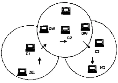
The protocol is based on the concept of clusters and cluster-heads. Routing is done via the cluster-heads and gateways, as shown by Figure 2.6, where GW is a gateway node, Cl, C2 and C3 are clusterhead to respective cluster, and MI and M2 are origin and destine node, respectively.

Figure 2.6: A CSGR path.

As show in Figure 2.6, a packet sent by a node is first routed to its clusterhead, and then the packet is routed from a clusterhead to a gateway to another clusterhead, and so on until the clusterhead of the destination node is reached. The packet is then transmitted to the destination.

2.4. AD­HOC MOBILE ROUTING PROTOCOLS 13

There can be some problem regarding the routing efficiency in CSGR. If the mobile riodes use CDMA/TDMA, theri it can take sorne time to get the permissions to send packets, as shown by Figure 2.7.

Cluster 1 Duaer2

Figure 2.7: Routing Iriemciency in CGSR.

We have two clusters, with node A in Cluster 1 and node C in Cluster 2 and node B in both clusters, also as a gateway. If node A wants to send packets in Cluster 1, it must get permission to do so. At the same time node B, the gateway, must select the same code as node A to be able to receive the packet from node A. Then node B rnust select the same code as node C and get permission to send in Cluster 2.

As we said earlier, routing is done with the help of clusters and gateways. But one important issue is how to define a cluster-head in a cluster and how select such a clusterhead, so a cluster head election algorithm is used. The algorithm used is the Lowest ID or Highest Connectivity algorithm. This assumes that initially clusters are formed based on lowest ID or highest connectivity. If a ClusterHead (CH) moves from a cluster A to another cluster

B, for example, then both clusters will give up its clusterhead appointment according to lowest ID or highest connectivity. In the saine time, nodes cletached from a cluster will recornputed their clustering according to lowest-ID or highest connectivity rnetric.

There are also some issues regarding cluster memberships, as cluster membership changes when cluster nodes migrate. Some iriteresting questions to solve are the following:

• how to derive unique cluster IDs

• how rnany nodes are allowable in a cluster.

14 CHAPTER. 2. WIKELESS AD­HOC NETWORKS

Wireless Routing Protocol (WRP)

This protocol was developed at U.C. in Santa Cruz, in 1995. Just like for the other men-tioned protocols, WRP simulations have been performed, but the protocol has never been implemented, [9].

WRP uses a distance-vector routing scheme, however it is a deviation from puré dis-tance vector routing. In WRP, routes are always available. Some nice features of the pro-tocol are that it is loop free and it also avoids the count-to-infinity problem by performing consistency checks of the reported predecessor information during routing updates. Some of the limitations of the protocol are the fact that it inaintains routing information among all the nodes, thus it has to maintain many tables and it uses periodic update messages.

The update messages can be of two types: periodic route updates, which maintain routing info and event-triggered updates which are generated in response to mobility. The information maintained in a node is stored in a couple of tables, like the Distance Table (DT), Routing Table (RT), Link Cost Table (LCT) and the Message Retransmission List (MRL).

2.4.2 Source­Initiated On­Demand Approaches

An approach that is different from table-driven routing is source initiated on-demand rout-ing. This type of routing creates routes only when desired by the source node. When a node requires a route to a destination, it initiates a route is found or all possible route perrnutations have been examined. Once a route has been discovered and established, it is maintained by sorne form of route maintenance procedure until either becomes inaccessible along every path from the source or the route is no longer desired, [4].

Associativity­Based Routing (ABR)

ABR was developed by C-K Toh at Cambridge University in 1996. The protocol is based on the concept of associativity, and new routing metrics are introduced, which are the longevity of a route (route relaying load) and the link capacity. The protocol is source-initiated thus there are no periodic route updates.

2.4. AD­HOC MOBILE ROUTING PROTOCOLS 15

Dynamic Source Routing (DSR)

DSR was developed in 1996 at CMU. As it is suggested in the ñame of the protocol, it is based on the concept of source routing. The protocol uses the shortest path as routing rrietric. Routes are discovered on-demand, and caching is also used, [10].

The protocol operates in two phases: first route discovery is performed and then route maintenance. During route discovery first a route request is broadcasted to all the nodes, and then the route reply containing the route-record is propagated back to the source. During the route maintenance phase orie has to take care of error packets and inform the source if necessary.

TORA ­ Temporally­Ordered Routing Algorithm

This protocol was developed at University of Maryland in 1996. It is clairned that it is implemented, but there are no experimental results reported, [11].

The protocol is on demand based; source iriitiated and uses the concept of link reversal. The concept used is based on building and maintenance of the 'height' metric, which aids routing. The 'height' is derived from the following valúes:

• logícal time of link failure

• unique riode ID

• ordering pararneter

• reflective bit indicator

The limitations of the protocol are that it is timing dependent, Information about adjacerit nodes must be maintained and potential oscillations cari occur. All this leads to a high protocol complexity. Due to its message passing nature it is suspected to have poor performance.

Similarly to the ABR protocol, TORA also has three phases of operation: the route discovery, route maintenance and route deletion. During the route discovery phase a Di-rected Acyclic Graph (DAG) has to be built from the destination. During route mainte-nance the DAG has to be rebuilt, while during route deletion a clear-packet is broadcasted.

AODV ­ Ad­hoc On­demand Distance Vector

16 CHAPTER 2. WIRELESS AD­HOC NETWORKS

vector is very weak, as it has changed from being table-driven to be on-demand. The implernentation is pending, and also a multicast versión is under evolution, [12], [13].

The protocol is essentially similar to DSR and it even has taken some part from ABR. Each node maintains its own sequence number. The protocol supports only symmetric links ancl rnay or may not use HELLO beacons. It operates by broadcasting RREQ messages until an interrnediate node has a route to the destination or until it receives a reply from the destination itself. There is no route selection capability, as the riode takes only the first route recorded by the first response orí the RREQ. Nodes not in the selected route do not particípate in route exchanges. Routes cari be truncated, and in this case the source must be informed to redo the RREQ. Routes expire on soft state.

ZRP­ Zone Routing Protocol

ZRP was developed at Cornell Uriiversity in 1998 by Z. Haas and M.Pearlamn. The al-gorithm combines the proactive and reactive approaches and is built upon the concept of zones. So in this way ZRP uses table-driven routing for nodes within a routing zone (this is also called IntrAzone Routing Protocol - IARP) and on-demand query for nodes outside a routing zone (IntErzone Routing Protocol - IERP). Every node defines a zone radius, but the problem is that it is hard to decide what is an appropriate zone radius that is good for all applications, [14] , [15].

Zone of Node Y

Zone of Node X

Zone of Node Z

2.5. QUALITY OF SERVICE (QOS) 17

Consider Figure 2.8, where it described the routing in ZRP, each node has routes to all other nodes in its owri zone, which is achieved by using IARP. Routes to nodes outside a zone can be requested usirig IERP by broadcasting the request to all border nodes. This process is called bordercasting.

ZRP's IARP relies on ari underlying neighbor discovery protocol to detect the presence and absence of neighboring nodes, and therefore, link connectivity to these nodes. Its main role is to ensure that each node within the zone has a consistent routing table that is up-to-date and reflects information on how to reach all other nodes in the zone.

IERP, however, relies on border nodes to perform on-demand routing to search for routing information to nodes residing outside its currerit zone. Instead of allowing the query broadcast to penétrate into nodes within other zones, the border nodes in other zones that receive this message will not propágate it further. IERP uses the bordercast resolution protocol.

Because parts of an ad hoc route are running different routing protocols, their charac-teristic will therefore be different. Sorne parts of the route is dependent on proper routing convergence, while the other part is dependent on how accurate the discovered interzone route is. This can rnake assurance of routing stability very difficult. Without proper query control, ZRP can actually perform worse than standard flooding-based protocols.

ZRP's route discovery process is, therefore, route table lookup and/or interzone route query search. When a route is broken due to node mobility, if the source of the mobility is within the zone, it will be treated like a link change event and an event-driven route updates used in proactive routing will inform all nodes in the zone. If the source of rnobility is a result of the border node or other zone nodes, the route repair iri the forrri of a route query search is performed, or in the worst case, the source node is informed of route failure, [4].

2.5 Quality of Service (QoS)

Quality of Service by the network is a guarantee to satisfy a set of predetermined service performance constraints for the user in terms of the end-to-end delay statistics, available bandwidth, probability of packet loss, and do on. The cost of transport and total network throughput may be included as parameters, [2].

The first essential task is to find a suitable path through the network, or route, between the source and destinatiori that will have the necessary resource available to rneet the QoS constraints for the desired service.

18 CHAPTER 2. WIRELESS AD­HOC NETWORKS

Chapter 3

Clustering in Ad­Hoc Networks

In order to rnairitain an Ad-Hoc network organizad, the network cari be divided in parti-tions denominated clusters of riodes. A Cluster is a group of similar thirigs (e.g., nodes iii telecornmunications systems), with similar characteristics. Then, protocol based on a cluster systerri consists of a set of rules applying cluster partition, where nodes have au-tonomously organized themselves to form clusters. Each cluster contains a clusterhead, zero or inore ordinary nodes and one or more gateways. Clusterhead are nodes whose main functions are transmissions and allocatiori of resources within the clusters, for example, it might issue tokens to potential transmitters, erriit busy tones when a transmission is in progress, or assign slots to specific transmitters and sessioris. Gateways connect ad-jacent clusters. A gateway may directly connect two clusters by acting as a member of both, or it may directly connect two clusters by acting as a member of one and forrning a link to a member of the other. Henee, the link-clustered architecture accommodates both overlapping and disjoints clusters, [5]. Figure 3.1 shows an example of a clustered network. With the link-clustered architecture, all cluster members are within one hop of the clusterhead and henee within two hops of each other. This arrangement provides low delay paths betweeri cluster members that may communicate frequently, and it places clusterheads in the ideal locations to coordinate transmissions arriong their cluster members. Clusterheads are distinct from gateways; henee, trióse for different clusters are separated by at least two hops. To establish a link-clustered control structure over a physical network, the nodes, [5],

• Discover neighbors to which they have bidirectional connectivity by broadcasting a list of those neighbors they can hear and receiving broadcasts from neighbors. • Elect clusterheads and form clusters.

• Agree on gateways between clusters.

CHAPTER 3. CLUSTERING IN AD­HOC NETWORKS

. CLUSTER __

~" CLUSTERHEAD

GATEWAY

ORDINARY NODE

Figure 3.1: Exarnple of cluster of Ad-Hoc network

3.1 Clustering Algorithm

The clustering algorithms to be discussed are completely distributed and adaptive. Henee, they are all suitable for highly dynamic wireless ad hoc networks. Distributed Mobility-Adaptive Clustering (DMAC) is based on the properties of the nodes, Distributed Dynamic Clustering Algorithm (DDCA) orí the properties of the links, and Access-Based Clustering Protocol (ABCP) performs access-based clustering.

3.1.1 DMAC Algorithm

The Distributed Mobility- Adaptive Clustering (DMAC) algorithm determines the cluster-heads not based orí the node ID, but based on the nodes' generic weights, which is a positive real number. In fact, the DMAC algorithm does not depend on how the weight is com-puted. Ideally, the weight captures the mobility and reliability of a node and characterizes the preferences on which a node is suitable as clusterhead, [16].

3.1. CLUSTERING ALGORITHM 21

The DMAC clustering algorithm works as follows. A node that is added to the network starts an iriitialization algorithm that determines it's role in the network, i.e. whether it should act as an ordinary node or a clusterhead. The decisión is based on its own and its neighbors' node weight. If the new node has a neighboring clnsterhead with a higher node weight, it decides to be ari ordinary node, joiris the cluster corresponding to that clusterhead and serids out a Join- message. Otherwise, it decides to become a clusterhead itself and serids out a ClusterHead- message, [16].

Thus, the neighbors get iriformed about the existence and role of a new node. The algorithm is message clriven and works consistently if every node stores its own identifier, weight and role as well as the identifiers, weights and roles of all its neighboring nodes. In order to be adaptive to the dynamics of the wireless network, every node has to react on both Join and Clusterhead rnessages as well as changes in the surrounding topology. Possible changes are for example the appearance and failure of links or the appearance of new nodes.

The detection of those events is the responsibility of an underlying protocol. In con-clusión, a stable, however temporary condition is reached if, first, every ordinary node is neighbor of at least one clusterhead, second, the affiliated clusterhead is the one with the highest weight, and third, two clusterheads are not neighbors. Figure 3.2 shows it algorithm.

3.1.2 ABCP Algorithm

An Access-Based Clustering Protocol (ABCP) designed for multi- hop wireless networks. Every ordinary node must be directly connected to the clusterhead. Basic design criteria were stable cluster structures and fast convergence, but moreover to keep the rnaintenance overhead as small as possible. The control channel plays an important role in this approach. The HELLO rnessages of the Médium Access Control (MAC) layer are included in the clustering process, [17], [18].

22 CHAPTER 3. CLUSTERING IN AD­HOC NETWORKS

Node compares its weight with neighbors

Is the node 's weight higher to its neighbors?

Node decides to become an ordinary node

Node sends out a Join message to clusterheads

\>

A clusterhead answers the request and node joins

to cluster

YES

Node decides to become a clusterhead

Node sends out a Clusterhead message to

other nodes

T

3.1. CL USTERING ALGORITHM

In order to maintain the original cluster as far as possible, clusterheads that are going to be inactivo send out a SUCCESSOR message. This message declares the node with the highest number of direct links as new clusterhead, i.e., the one with the highest connectivity. Another refinement is that clusterheads that have no ordinary node in their cluster also send out a REQUEST TO JOIN message. If there exists at least one clusterhead this node is directly connected to, it will receive a HELLO message, send out a JOIN message and become an ordinary node. Figure 3.3 shows it algorithm.

Node sends out a Request to join message to the clusterhead, and

initiate a timer

Is a Helio message received from any clusterhead in a certain

time?

Node sends out a Join Message to respective clusterhead and adds to it

Node sends a Helio message and decides to

become a clusterhead

Figure 3.3: ABCP Flowchart

3.1.3 Application of the clustering algorithms to the sample sce­

nario

24 CHAPTER3. CLUSTERING IN AD­HOC NETWORKS

upon three basic changes in the topology: appearance of a new node, link failure and occurrence of a new link, [6], [16], [17], [18]. Figure 3.4 shows the initial network, where we have the link probabilities, identification and weight of each node in order to apply algorithm review before.

Link ­\ ­> Probability

>Node"s weight

Node's Identification

Figure 3.4: Initial Ad hoc Network

New Node

Figure 3.5 shows the sample network with an additional node 15 that was just activated. It has a node weight of 29 and is connected to both node 4 and node 5. Figure 3.5a shows the clustering result according to DMAC, Figure 3.5b according to ABCP. In the following, the reaction of the three presented clustering algorithms on this new node event will be described, [6], [16], [17], [18].

DMAC. The cluster formation completely changes because of the insertion of just one node, as shown in Figure 3.5a. The reason for that is that a new node does not accept a clusterhead with lower weight. Moreover, a chain reaction along nodes 15, 4, 8, 1,2 occurs. The term chain reaction describes the fact that along a certain path, the roles of ordinary nodes and clusterheads invert. A chain reaction will always occur if (1), a new node has a higher weight than his clusterhead, (2), clusterheads and ordinary nodes appear alternately along a path, (3), the next node in the path has a lower weight than the node before, and (4), there is no ordinary node in the path having a clusterhead with higher weight than its predecessor in the path.

3.1. CL USTERING ALGORITHM

a)

Figure 3.5: a) New Node, DMAC Algorithm. b)New Node, ABCP Algorithm. occur. ABCP tends to form new clusters, changes are kept more locally and chain reactions don't occur. Henee, it is useful that in the refinements of ABCP, isolated clusterheads seek to join other clusters.

Link Failure

Lets consider the failure of the link between nodes 4 and 8. Figures 3.6a to 3.6b show the corresponding clustering by the different algorithms.

a)

Figure 3.6: a) Link Failure, DMAC Algorithm. b)Link Failure, ABCP Algorithm.

26 CHAPTER 3. CLUSTERING IN AD­HOC NETWORKS

results in a severe change of the cluster structure, compare Figure 3.2a and Figure 3.3b. This happens even as there is only one link failure in an área with relatively high connectiv-ity. However, this is due to the fact that a link between an ordinary node and a clusterhead failed. If, instead, a link between two ordinary nodes would fail, a stable clustering would be maintained.

ABCP. The only change in the cluster structure upon the link failure using ABCP is that node 8 now belongs to a different cluster, the one of node 1, as node 8 could receive node l's HELLO message. The approach is obviously stable in cases where a second neighboring clusterhead exists.

New link

As one might expect, new link events due to the fact that mobile stations get connected that have not been connected before do not cause severe clustering changes. However, the DMAC algorithm does not allow two clusterheads to be neighbors. This is why in the following example it DMAC is the only approach that will change the cluster structure after a new link is available, see figures 3.7a and 3.7b, [6], [16], [17], [18].

Figure 3.7: a) New Link, DMAC Algorithm. b) New Link, ABCP Algorithm.

3.2 DDCA Algorithm

3.2. DDCA ALGORITHM

algorithm works with message driven and needs no periodic re-clustering but is

continu-ously executed by all active nodes. The DDCA approach uses a so called

 (a, i)

-criterion

for clustering (edge based). The criterion describes a probabilistic bound, a, on the

avail-ability of paths in the corresponding cluster over a certain time ¿, [6]. Figure 3.8 shows a

flowchart with DDCA algorithm.

New node sends a Join Request Message

New node receives response ?

New node becomes an orphan cluster and clusterhead

New node decides to joln the cluster provlding the highest valué of path with respect to the bound

Figure 3.8: General flowchart for DDCA Algorithm

According to Figure 3.8 , a new node seeking a cluster to join sends out a JoinRequest

message. If it does not receive any responses, it basically builds a new cluster and becomes

clusterhead. This process is a little more involved as a deferral algorithm is used to handle

situations with simultaneously broadcasted JoinRequest messages. If the new node upon

sending a JoinRequest receives one or more JoinResponse messages before its JoinTimer

runs out, it decides to join the cluster providing the highest (a, í)-value. This valué has to

exceed the mínimum required valué

 (a, t)

threshold, otherwise the JoinResponse is ignored.

The cluster strength, seen by a node m and given by the

 (a, t)­

valué, is a measure of the

availability of a path from node m over some initial hop node n to the clusterhead of the

corresponding cluster.

3.2.1

( a , t )

 Cluster Framework

28 CHAPTER3. CLUSTERING IN AD­HOC NETWORKS

aggregation achieves the effect of making a large network appear much smaller from the perspective of the routing algorithm. Cluster-based routing in ad-hoc networks can also make a large network appear smaller, but more importantly, it can make a highly dynamic topology appear much less dynamic. Unlike the cluster organization of a fixed network, the organization of an ad-hoc network cannot be achieved ofnine. The assignment of mobile nodes to clusters must be a dynamic process wherein the nodes are self-organizing and adaptable with respect to node mobility. Consequently, it is necessary to design an algo-rithm that dynamically implements the self-organizing procedures in addition to defming the criteria for building clusters, [3].

The objective of the (a, í) cluster framework is to maintain an effective topology that adapts to node mobility so that routing can be more responsive and optimal when mobility rates are low and more efficient when they are high. This is accomplished by a simple distributed clustering algorithm using a probability model for path availability as the basis for clustering decisions. The algorithm dynamically organizes the nodes of an Ad-Hoc network into clusters where probabilistic bounds can be maintained on the availability of paths to cluster destinations over a specified interval of time.

The (a, í) cluster framework can also be used as the basis for the development of adap-tive schemes for probabilistic QoS guarantees in Ad-Hoc networks. Specifically, support for QoS in time-varying networks requires addressing:

• Connection-level issues related to path establishment and management to ensure the existence of a connection between the source and the destination.

• Packet-level performance issues in terms of delay bounds, throughput, and acceptable error rates.

3.2.2 (a,

t)

 Cluster Characterization

The basic idea of the (a, i] cluster strategy is to partition the network into clusters of nodes that are mutually reachable along cluster internal paths that are expected to be available for a period of time t with a probability of at least. The unión of the clusters in a network must cover all the nodes in the network, [3].

Definition 1: Let P^n(t) indícate the status of path A; from node n to node m at

time í, P^n(t) = 1 if all the links in the path are active at time t , and P^n(t) = O if one

or more links in the path are inactive at time í, Figure 3.9 shows this notation, here 1 and 2 are the possible paths from the origin node to the destination node, note that path 2 has an intermediate node r, while path 1, does not. The path availability W^¡n(t) between two

3.2. DDCA ALGORITHM 29

Inactive Link

Figure 3.9: Notation to Definition 1.

,„(*) = !)• (3-1)

Definition 2: Let W^<n(t} be the path availability of path k from node n to node m

at time t. Path A; is defined as an (a,t) path if and only if,

W£,B > «• (3­2)

Definition 3: Node n and node m are (a, í) available if they are mutually reachable

over (a, í)paths.

Definition 4: An (a, í)cluster is a set of available nodes. Definition 4 states that

every node in an (a, í)cluster has a path to every other node in the cluster that will be available at time (¿o + t) with a probability a. The cluster characterization, as previously defined, requires a model which quantifies the (a, í) path availability as given in Definition 1. Path availability is a random process that depends upon the mobility of the nodes which lie along a given path. Consequently, the mobility characteristics of the nodes play an important role in the characterization of this process.

3.2.3 Clustering Algorithm

Two key requirements motívate the design of a successful dynamic clustering algorithm, [3],

• The algorithm should achieve a stable cluster topology.

30 CHAPTER3. CLUSTERING IN AD­HOC NETWORKS

propagates routing Information from nodes that do belong to its cluster is processed and disseminated. No centralized control over the clustering process is required. Nodes can asynchronously join, leave, or créate cluster, [1].

In this Algorithm, we have four parameters to make a cluster: • Node Activation

• Link Activation • Link Failure • Node Deactivation

We can describe these parameters in a flowchart as that of Figure 3.10, 3.11 and 3.12

Node Activation: The primary objective of an activating node is to discover an ad-jacent node and join its cluster. In order to accomplish this, it must be able to obtain topology information for the cluster from its neighbor and execute its routing algorithm to determine the (a, i) availability of all the destination nodes in that cluster.

The source node can join a cluster if and only if all the destinations are reachable vía (a, i) paths. Such a cluster is referred to as a feasible cluster. The source node will continué checking each neighbor in sequence until it finds a feasible cluster or runs out of neighbors. If the source node is unable to join a cluster, it will créate its own cluster, referred The cluster-join action is achieved asynchronously without any additional internodal coordination. The source node sets its node's Cluster Identifier Number (CID) to equal the CID of the cluster it is joining, and it generates its own routing update that is broadcast to its neighbors, [3]. Recognizing their own CID's in the routing update, those neighbors that are members of the target cluster process the source node's routing update. In doing so, the routing protocol automatically adds the source node as a destination in their respective routing tables, which infers cluster membership.

If the source node's network-interface layer protocol detects no adjacent nodes, or its attempts to join an adjacent cluster fail due to cluster infeasibility, the cluster algorithm generates and sets a globally unique CID that will be used in subsequent neighbor greeting exchanges. In this orphaned state, the (a, í)criteria is trivial because the path availability of the source node to itself is always one. In order to periodically reattempt to join a neighboring cluster, the node's timer is set to the valué of the system parameter. Figure 3.10, shows this process.

3.2. DDCA ALGORITPIM 31

YES

Node state = Unclustered

Node checks each neighbor node to find a cluster to addition

YES

New node state = Clustered

Node pass to state Orphan cluster

NO

32

CHAPTER 3. CLUSTERING IN AD­HOC NETWORKS

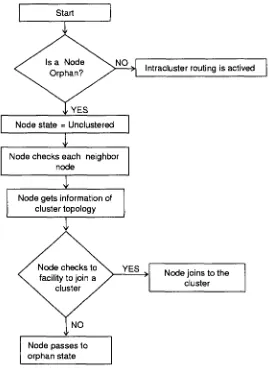
to join a cluster. In order to receive cluster topology Information from its new neighbor, the orphan node must temporarily reset its CID to indícate its unclustered status. Only information received from nodes that are in the same cluster as a destination or in the unclustered state are passed by the cluster algorithm protocol to the routing layer.

Thus, by changing its CID, the orphan node triggers the transmission of routing updates from its neighbor. Upon receiving the cluster topology information, the node evaluates cluster feasibility and either joins the cluster or returns to its orphan cluster status, depending upon the outcome of the evaluation. Figure 3.11, shows this process.

Start

Intracluster routing ¡s actived

YES

Node state = Unclustered

Node checks each neighbor node

Node gets information of cluster topology

Node checks to facility tojoin a

cluster

Node passes to orphan state

Node joins tothe cluster

Figure 3.11: Link Activation Flowchart

3.3. TRELLIS ALGORITHM FOR AD­HOC NETWORKS

33

if the link failure has caused the loss of any (a,í)paths to destinations in the cluster. A node's response to a link failure event is twofold. First, each node must update its view of the cluster topology and reevaluate the path availability to each of the cluster destinations remaining in the node's routing table. Second, each node forwards information regarding the link failure to the remaining cluster destinations. Each node receiving the topology update reevaluates its (a,t)paths as if it had directly experienced the link failure. When evaluating path availability to destination nodes within the cluster following a topology change, it is necessary to adjust the timing parameter to reflect that the timer has not yet expired. Use of the full valué of would unnecessarily penalize the nodes by requiring a path availability that is higher (further out in time) than required by the cluster criteria. Thus, the estimated availabilities will reflect the probabilities evaluated at the máximum time for which this node has already made its probabilistic guarantee.

Using the topology information available at each node, the current link availability information is estimated, and máximum availability paths are calculated to each destination node in the cluster. If the node detects that a destination has become unreachable, then the node assumes that the destination has deactivated or otherwise departed from the cluster. In this case, the destination is removed from the node's routing table and will not be considered further in the evaluation of (a, í)paths. If a node detects that any of the remaining cluster nodes are connected within the cluster but not (a, í)reachable, it will voluntarily leave the cluster. A node leaves a cluster by sending a routing update to its neighbors that indicates that the status of all its links are down or equivalently an infinite distance to itself. It then resets its own CID to the unclustered valué and proceeds according to the rules for node activation. No further action is required following a link failure if the node successfully evaluated (a, í)paths to each destination in the cluster,[3].

3.3 Trellis Algorithm for Ad­Hoc Networks

In order to analyze some concepts about quality and connectivity in Ad-Hoc networks, we need to find paths efficiently and easily to evalúate the performance measures. To use a Trellis algorithm is an alternative to pursue those objectives. In this case, we change the form to find the path cost, because we are using probabilities in the links cost; this change will be explained in the following sections. Now, we introduce some theoretical concepts and establish the notation and terminology, [19].

3.3.1 Graph Modeling

34 CHAPTER 3. CLUSTERING IN AD­HOC NETWORKS

If one or more paths are broken, nodes update their

routing tables

Origín node gets destination node?

Node is removed from routing table.

Destination node does not have signal from each other into its cluster , thus it leaves voluntarily from the cluster and it send routing tables with infinite distances

3.3.

 TRELLIS ALGORITHM FOR AD­HOC NETWORKS

each link is an ordered pair.

Consider a node S (origin) and a destination node Z, we define a Trellis as a direct graph G — (V, E] with nodes and directed links that satisfies the following conditions:

• The node set V s, z is partitioned into L subsets Vi,V2,..,VL such that the cardinality

of each set i is \ Vi |= H, I < i < L, where H is the amount of nodes in each subset. • Links connect nodes only of consecutive subsets V/ and V/+1 , for example, if (vi, Vj) 6

E, then v^ e V¡ and Vj e V/+1, i < z < L .

• It has two more nodes s e V0 and t e VL+1 such that (s,Vi) e E for every v¡ € VL

and  ( v j , z ) e E for every w¿ e V¿, 1 < ¿, j < //.

Figure 3.13 shows the parameters just described, where s is an origin node and z is a destination node. A walk on a trellis is an alternating sequence of nodes and links, i.e.,

P = [vi, (vi,v2),V2,..., (vk­i,Vk),Vk\­ The length L(P) of a walk is the path of links in it.

A path is a walk in which all nodes are distinct.

L=5

Figure 3.13: A X-Trellis graph with L=5, //=4

3.3.2 Link and Path Cost

Another parameter that needs to be studied in each link (t>¿, Vj) e E of a trellis graph, t>¿ e

Vi and Uj e V/+i, is the link cost and denoted G(VÍ,VJ), I < i,j < H. Let P = {vi,v2, Vk}

be a path in a trellis graph. Consider G(VÍ,VJ) as the cost of  ( i , j ) G E, then the cost, c(P), of a path P through the Trellis is defined as

36 CHAPTER 3. CLUSTERING IN AD­HOC NETWORKS

The shortest path from node t>¿ to node Vj is a path P = {t»¿,f¿+i, Vj} with mínimum cost.

For this work, as a contribution of this thesis, we are using probabilities as cost of links, therefore we change Equation (3.3) as

c(P)= n c(^). (3.4)

Vi,Vj£P

3.3.3 Algorithm Net to Trellis

Consider the network topology G = (V, E, c), where c is the cost function from the link set

E to a real number. The algorithm consists of the next steps, [19]:

1. The first step in the transformation process toward'the trellis graph is to partition, with respect to a particular node, the node set of the network into adjacency- levéis. By definition, this partition places the nodes of the network at vertical levéis according to their distances.

2. In this step, we disconnect the network into two subnetworks G' and G". Network G" contains all the nodes and links except the destination node t and the links incident to it. Network G" contains the nodes in set{í} U N(t) and all the links with end-nodes

t and x, where x € N(t).

3. If now after step 1 and 2, we have any "vertical" links in G", for example two nodes connected by a link belonging to the same level, we apply two specific operations which eliminate "vertical" links. These operations are based on the addition of dummy nodes and 0-cost links, in such a way that the path cost is preserved.

4. In this step, we merge the resulting graph G' from step 3 with the graph G" by adding (if necessary) dummy nodes and 0-cost links.

5. Now, if necessary, to complete the trellis graph, we introduce more dummy nodes, but with infinite link cost.

Definition: Let x, y be two nodes of consecutive levéis which are connected by a link. The s-cost of link (x, y) is defined to be mínimum cost of the path from s to y through node x , i.e., the cost of the path P = {s, , x, y} , and is denoted by <f>(x,y)

Operation Pl: Let G(V, E, c) be a network partitioned into adjacency-levels and let

3.3. TRELLIS ALGORITHM FOR AD­HOC NETWORKS 37

before the application of the Operation Pl the link vertical (x, y) has only link cost, while after the operation it gains link s-cost.

We can see in Figure 3.14a that, links cost are positive integer numbers, and the link cost when a dummy node is presented is zero, but in this thesis we are using probabilities as links cost, therefore the link cost when a dummy node is presented is one (1) to no affect the path cost, explained in the section before. This is a contribution of this work.

Let x be the node satisfying the following properties

min{</>(a;, v] : v e AL(s, / — !)}> min{(f)(y, u) : u e AL(s, I — 1)}, E <f>(x,v)> E <í>(y,u)­

v&N(x)CiAL(s,l-l) u£N(x)nAL(s,l-l)

Then, replace node x with a dummy node x', move node x into level I + 1 and update the following parameters

w(x,x') = O,

<j)(x,x"} = min{<j)(x',v) : v E AL(s,l - 1)},

(j>(x, y) = min{0(o;, v) : v e AL(s, / — !)} + c(x,y).

Operation P2: Let G(V, E,c) be a network and let £ be a node at level / which, after operation Pl, remains without neighborhoods in level / — 1, i.e.,N(x) n AL(s, I — 1) = 0. Then, move node x into level / -f 1 and update the following parameter,

<f)(x, y) = min{(f)(x, v) : v e AL(s, /-!)} + c(x, y}.

Figure 3.14b shows the resulting network topology when Operation Pl is applied to node x. Both links (z,x) and  ( y , x ) have now link s cost.

In summary we have the formal listing to apply the algorithm described above. 1. Partition the node set of the network G(V, E, c) into adjacent-level sets, with respect

to origin node s e V . That is, the nodes of the network are placed at levéis according to their distances from s; the origin s is placed at level 0.

2. Disconnected the network into two subnetworks G' and G"', where G'contains all the nodes and links except the destination node t and the links incident to it, while

G" contains the nodes in set {z} U  N ( z ) and all the links of the form (x,z), where

x E  N ( z ) .

38 CHAPTER 3. CLUSTERING IN AD­HOC NETWORKS

3(9)

2(5)

Dummy Node

2(7)

4

<8) ~ LinkCost ­­ — ­ 4(8) ^ ... ID Node

5­cost of the link

a) Illustration of Application of the Operation Pl

0(5)

1 ( 4 )

b) Illustration of Application of the Operation P2

3.3. TRELLIS ALGORITHM FOR AD­HOC NETWORKS 39

4. Merge the resulting network from step 3 with the network G" by adding dummy nodes and 0-cost links.

5. Complete the trellis structure by adding oo -cost links. Figure 3.15 shows the flowchart about Trellis Algorithm.

Partition the node set of the network G(V,E,c) into adjacent level sets, according to origin node.

Disconnect the network into two (sub) networks G' and G".

Are there vertical links in the network

G'?

Apply operaüons Pl and P2

Complete the network G' with G" and adding dummy nodes.

Complete the Trellis structure

Figure 3.15: Trellis Algorithm Flowchart

3.3.4 Example applying Trellis Algorithm

40 CHAPTER 3. CLUSTERING IN AD­HOC NETWORKS

According to section 3.3.3, where dummy links had a zero valué due to they are not probabilities, but in this case dummy links have one-valué because we are using probabilities as link costs. See Figure 3.16, where pi, p2, Ps are link probabilities.

Figure 3.16: Transformation from normal network to Trellis Graph

In Figure 3.16 we observe the transformation form a normal Network to Trellis Graph. For this transformation, we apply the steps described before in this chapter, but applying the new parameters for dummy link and link cost. For example if we consider network in Figure 3.17, and we try to convert it to a Trellis Graph to find the k-paths. Figures 3.16, 3.18, 3.19 and 3.20 show these.

If we take each cluster and apply the Trellis Algorithm we obtain an easily form to find fc-paths into each cluster, and after that we take each cluster as a node and apply the algorithm again.

According to Figure 3.18 in a) Step 1 and 2 from the Trellis algorithm to Cluster A, b) Step 3 and 4 from Trellis algorithm to Cluster A, c) Step 5 from the Trellis algorithm to Cluster A. Now, we are applying this method in all cluster, separated, we can see Figure 3.19 for cluster B, and Figure 3.20 for cluster C.

Now, we need to know paths between clusters, so we apply again the trellis algorithm, but now we take the border nodes in the cluster as nodes in the network, in Figure 3.21 we can see that.

Now, applying Equation (3.4), we can obtain all possible paths from origin to desti-nation, according to the procedure developed before. Figure 3.22 we can see it.

Figure 3.22 shows the best path from node 5 to node 3 and pass trough nodes 4, 8, 12, according to equation (3.4), where,

c(P] = (0.87)(1.00)(0.7)(0.5)(1.00)(0.7)(1.00) = 0.21924.

3.3. TRELLIS ALGORITHM FOR AD­HOC NETWORKS 41

ünk Probability

Node's Identification

Figure 3.17: Initial Ad-Hoc Network.

0.72

0.75

10

0.87

4.9

0.72

42 CHAPTER 3. CLUSTERING IN AD­HOC NETWORKS

0.7

12

0.7

0.55

0.65

Figure 3.19: Trellis Algorithm applied to cluster B

1 2

Figure 3.20: Trellis Algorithm applied into cluster C

B