STOCHASTIC MODELING OF HYDROMETEOROLOGICAL EXTREMES AND THEIR POSSIBLE RELATION WITH GLOBAL CHANGE
A Master Thesis Presented by THOMAS ROSMANN
Directed by
Submitted to the Maestría en Hidrosistemas of the Pontificia Universidad Javeriana in fulfillment
of the requirements for the degree of
MAGISTER EN HIDROSISTEMAS
iii
ACKNOWLEDGEMENTS
At the moment of completion of this document, I would like to take the time to express my gratitude to some of the people who helped me make all this possible.
First and foremost, I want to thank my tutor Efraín Domínguez, whose everlasting patience and compassion were some of the driving forces of this investigation. Not only his motivation, but also his constant availability at any moment made it possible to eliminate the doubts I had by answering all my questions and always giving me new ideas, which is why this work resulted the way it did. Elaborating this thesis with his guidance I learned a lot, not only from the technical side but also human quality.
Also, I would like to thank Andrés Torres for facilitating me to enter the masters program and overcome all the initial problems I had. It was also due to his help and to a big part to Nelson O ego ’s generous job offer at the Geophysics Institute that I could continue my studies after the first semester.
I would like to thank all of my colleagues in the masters program, especially Hugo and David for initially including me into the group of students, always being there to help and for their good company. Also, Natalia, Alejandra, Jorge and Felipe for accepting me for who I am and spending a lot of great moments with me. I am lucky to say that I found such good friends and the time I spent in the masters program was one that I will always remember with a smile.
Thanks to all the other faculty staff and professors that shared their knowledge and supported me when I had needed it with an almost completely new topic, a new culture and language, and helped me develop myself thanks to the projects in which I was allowed to participate. Finally, I would like to thank Sandra for supporting me all this time, for always offering help and good advice to continue working hard. Also her family who opened their doors to me, made me feel welcome and supported me whenever I needed it.
iv
AGRADECIMIENTOS
En el momento de terminar este documento quiero tomar el tiempo para expresar mi gratitud a algunas de las personas que ayudaron durante el camino para llegar a este punto.
Primero de todo, quiero agradecerle a mi director Efraín Domínguez por su infinita paciencia conmigo y su compasión, las cuales fueron unas de las fuerzas más importantes que ayudaron a seguir con el trabajo. Se debe a su motivación y constante disponibilidad en cualquier momento para aclarar todas mis dudas y darme consejos y nuevas ideas que el trabajo resultó de la forma como está. Elaborando éste trabajo de grado con él aprendí mucho, no solamente del lado técnico sino también de la calidad humana.
También quiero decirle gracias al ingeniero Andrés Torres, quien fue la persona que me hizo posible entrar a la Maestría de Hidrosistemas a pesar de todos los problemas que se me presentaron al principio. También se debe a él y por gran parte a la oferta de trabajo generosa del profesor Nelson Obregón en el Instituto Geofísico que pude seguir con la carrera después del primer semestre.
Quiero agradecerles a todos mis compañeros de la maestría, especialmente a Hugo y David por introducirme inicialmente al grupo de estudiantes, por siempre estar a la orden para ayudar en todo cuando lo requería y por su buena compañía. También gracias a Natalia, Alejandra, Jorge y Felipe por aceptarme como soy y pasar tanto tantos buenos momentos juntos. Puedo considerarme afortunado de haber conocido amigos tan buenos que fueron una de las razones principales por las cuales siempre voy a recordarme del tiempo de la maestría con una sonrisa. Gracias a todos los miembros de la facultad y los profesores que compartieron su conocimiento y me apoyaron en tiempos en que se me hizo difícil entender un tema casi completamente desconocido, una nueva cultura y un idioma diferente, y que ofrecieron a desarrollarme en los proyectos en los cuales tuve la oportunidad de participar.
Finalmente, quiero agradecerle a Sandra por siempre apoyarme en todo y ofrecer su ayuda y buenos consejos para seguir trabajando duro. También a su familia que me abrió las puertas, me hicieron sentir bienvenido y me brindaron su apoyo siempre que lo necesitaba.
v
TABLE OF CONTENTS
Page
1 INTRODUCTION ... 1
2 CONCEPTIONAL DOMAIN... 5
2.1 Fundamentals concepts ... 5
2.1.1 Probability ... 5
2.1.2 The Axiomatization of Kolmogorov ... 5
2.1.3 Random variables ... 6
2.1.4 Random processes ... 8
2.2 Extreme Events ... 10
2.3 Statistical Methods ... 11
2.3.1 PDF Fitting and Kolmogorov goodness of fit test ... 11
2.3.2 Mann-Kendall trend test ... 12
2.3.3 Thomas Algorithm ... 13
2.3.4 Multiple Regression Analysis ... 13
2.3.5 Kullback-Leibler divergence criteria... 14
2.4 Computational Tools ... 15
2.4.1 Python programming language ... 15
2.4.2 ArcSWAT ... 16
2.5 Data collection... 17
2.5.1 Hydrometeorological data ... 17
2.5.2 Geospatial data ... 20
2.6 Study areas for extreme event analysis ... 21
2.6.1 Enns River Basin (Austria) ... 22
2.6.2 Upper Magdalena River Basin (Colombia) ... 24
2.6.3 Upper Great Miami River Basin (USA) ... 25
2.6.4 Brisbane River Basin (Australia) ... 27
3 WORLDWIDE TREND ANALYSIS ... 29
3.1 Background and methodology ... 30
vi
4 STOCHASTIC MODEL APPROACH ... 39
4.1 Stochastic Hydrological Modeling ... 40
4.1.1 Complex systems ... 40
4.1.2 The Langevin Equation ... 40
4.1.3 The Fokker-Planck-Kolmogorov (FPK) Equation ... 41
4.1.4 Relationship between Langevin and FPK equation ... 43
4.1.5 Determination of Markov process structure ... 44
4.2 Implementation of the Fokker-Planck-Kolmogorov Equation ... 47
4.2.1 Finite-difference system ... 47
4.2.2 Optimization of model parameters ... 51
5 DATA PREPARATION AND RESULTS ... 53
5.1 Initial conditions ... 53
5.2 Optimization of model parameters ... 58
5.3 Relation of model parameters to physical properties ... 65
5.4 Supervised optimization with fixed model parameters ... 70
5.5 Application of the model to estimate the change of extreme regimes... 72
5.5.1 Simulation with external parameters ... 73
5.5.2 Simulation with internal parameters ... 75
5.5.3 Simulation with external and internal parameters ... 78
6 CONCLUSIONS ... 81
REFERENCES ... 84
Annex A: List of data sources ... 88
vii
LIST OF FIGURES
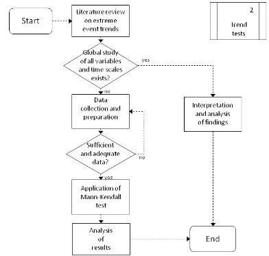
Figure 1. Schematic outline of the proposed work ... 4
Figure 2. Bundle of realizations and probability density functions of a random process: monthly mean discharges, Pte. Balseadero station, Colombia ... 9
Figure 3. Location of the study areas ... 22
Figure 4. Illustration of the Enns River basin ... 23
Figure 5. Illustration of the Upper Magdalena River basin... 25
Figure 6. Illustration of the Upper Great Miami River basin ... 26
Figure 7. Illustration of the Brisbane River basin ... 28
Figure 8. Schematic outline of worldwide trend analysis ... 29
Figure 9. Location of the discharge stations used in trend analysis ... 32
Figure 10. Location of the precipitation stations used in trend analysis... 32
Figure 11. Location of the temperature stations used in trend analysis ... 33
Figure 12. Results showing statistically significant trends for mean values ... 34
Figure 13. Annual statistically significant trends in minimum temperature ... 34
Figure 14. Results showing statistically significant trends for extreme values ... 35
Figure 15. Trends in discharge maxima ... 35
Figure 16. Trends in annual precipitation ... 36
Figure 17. Histograms of coefficients of variation for different variables ... 37
Figure 18. Schematic outline of the development of the stochastic model ... 39
Figure 19. Drift and diffusion of probability density functions ... 43
Figu e . Dete i atio of the p o esses’ oss o elatio i the E s a d Uppe Magdale a basins ... 45
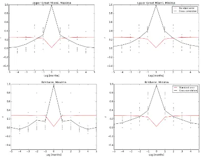
Figu e . Dete i atio of the p o esses’ oss o elatio i the Uppe G eat Mia i a d Brisbane basins ... 46
Figu e . Dete i atio of the p o esses’ oss o elatio fo the C o odile Ri e asi ... 46
Figure 23. Scheme of an absorbing boundary ... 50
viii Figure 25. Probability density functions of the random variables in the Upper Magdalena River
basin ... 55
Figure 26. Probability density functions of the random variables in the Upper Great Miami River basin ... 56
Figure 27. Probability density functions of the random variables in the Brisbane River basin ... 57
Figure 28. Schematic outline of model calibration ... 58
Figure 29. Results of optimization in the Enns River basin ... 61
Figure 30. Results of optimization in the Upper Magdalena River basin ... 62
Figure 31. Results of optimization in the Upper Great Miami River basin ... 63
Figure 32. Results of optimization in the Brisbane River basin ... 64
Figure 33. Numerical diffusion using the explicit scheme ... 65
Figure 34. Correlation between discharge maxima and precipitation ... 66
Figure 35. Correlation between discharge minima and precipitation... 68
Figure 36. Schematic outline of model evaluation ... 73
Figure 37. Simulation of the model applying changes to external parameters in the Upper Great Miami basin ... 75
Figure 38. Simulation of the model applying a change of -10% to internal parameters in the Enns basin ... 77
Figure 39. Simulation of the model applying a change of +10% to internal parameters in the Upper Magdalena basin ... 78
ix
LIST OF TABLES
Table 1. Hydrometeorological stations used in the Enns River basin ... 24
Table 2. Hydrometeorological stations used in the Upper Magdalena River basin ... 25
Table 3. Hydrometeorological stations used in the Upper Great Miami River basin ... 27
Table 4. Hydrometeorological stations used in the Brisbane River basin ... 28
Table 5. Comparison of the magnitudes of values resulting from drift (A) and diffusion (B) components ... 48
Table 6. Best probability density function fit for each random variable in the Enns River basin 54 Table 7. Best probability density function fit for each random variable in the Upper Magdalena River basin ... 55
Table 8. Best probability density function fit for each random variable in the Upper Great Miami River basin ... 56
Table 9. Best probability density function fit for each random variable in the Brisbane River basin ... 57
Table 10. Example of optimized parameters using different initial guesses ... 59
Table 11. Lag times and method with the highest correlation between discharge maxima and precipitation values for each basin ... 67
Table 12. Correlation between discharge minima and monthly mean temperature for all basins ... 69
Table 13. Initial guesses used in the 3 runs of supervised optimization ... 70
Table 14. Results of multiple regression analysis between the model parameters and the coefficients of variation and skewness ... 72
Table 15. Averages of Kullback-Leibler divergences between present and future simulations of all PDF translations of each basin, applying changes to external properties ... 74
Table 16. Averages of Kullback-Leibler divergences between present and future simulations applying changes to internal properties ... 76
1
SECTION 1
INTRODUCTION
In recent years and decades, the topic of global climate change has become one of the most controversial and heavily discussed. By now, scientists have found sufficient proofs that the global climate has experienced abrupt changes in the last decades, since the mid-19th century, but with the strongest increase from the 1950s onwards (IPCC, 2013). The most obvious characteristic is global warming, which most certainly influences on other variables as well, which was proven for some areas in previous studies (Wang et al., 2009; Woo et al., 2008). The moments when the existence of global change calls the attention of people most drastically is when emergencies occur as a result of it. For a large number of events in the recent past, news about human tragedies as results of climatic phenomena have reached the public, such as for example hurricane Katrina in New Orleans in 2005, typhoon Haiyan on the Philippines in 2013, severe floods in Australia and large parts of central Europe in 2011 and 2013, respectively, an extreme cold wave in North America at the beginning of 2014 or a large number of extensive droughts in India, for example in 2013, and eastern Africa, especially in the years of 2008 to 2009 and 2010 to 2011, just to name a few. In all these cases, a connection to global change was established in the media and discussed in public and politics.
In its recently released Fifth Assessment Report (IPCC, 2013), the Intergovernmental Panel on Climate Change (IPCC) mentions that it can confidently be stated that temperature has been rising steadily since the 1950s and that the change in precipitation over the global land mass is characterized as being of medium strength. However, it is only worded as likely that changes in extreme events have occurred since the beginning of observation in about 1950. Among these extreme events are increases of heat waves on a global scale and heavy rainfall events in North America and Europe.
Another recently published report, the United Nations’ World Water Development Report 2014 (UNESCO, 2014), predicts an increase in worldwide water consumption of about 55% until 2050, with which energy and alimentation demand are closely related. Just this one fact states the importance to study profoundly the state of water resources and any impacts that influence on them. One of these influences is the occurrence of extreme events, which can cause a variety of problems in water supply, including shortages, contamination or damages to infrastructure, among others.
2 frequent one. Both linear and nonlinear trends have been applied, as well as flood frequency analysis. Results of these studies in many cases indicate intensifications of the extreme events, but also state that the period that reliable hydrometeorological data is too short to prove the existence of changes (Bordi et al., 2009). A more detailed study of previous works that investigated the topic of trends in hydrometeorological time series will be given in section 3. Other studies treated with the topic of occurrence of extreme events, such as floods, which seemed to have increased over the last years (Kundzewicz et al., 2013), or relate extreme events or trends in hydrometeorological time series to the level of CO2 emissions or microclimatological indices (Hirsch and Ryberg, 2012; Moreno, 2011), but do not always succeed to prove the impact of these indicators.
In order to prevent harm to persons and impacts on structures and ecosystems, various measures on the administrative level have been taken. One of many examples is the Floods Directive of the European Parliament (European Parliament, 2007), which has been applied to national laws of the member states of the European Union and triggered a large number of research projects related to the topic.
But not only on the administrative level, also in many other fields of economy or research, the topic of extreme events causes an increased interest. Needless to say, the impact of these events are crucial for the work of insurance companies (Spekkers et al., 2013), but also in many other diverse fields research has been conducted, for example for the design of urban drainage systems (Smith et al., 2002), the risk of extinction of species due to extreme events (Colomer et al., 2014) or the evaluation of irrigation pricing during drought periods (Nikouei and Ward, 2013), just to name a few.
3 characteristics of hydrological processes (Naidenov and Podsechin, 1992; Naidenov and Shveikina, 2005, 2002), as well as Koutsoyiannis et al. (2008) in the Nile River basin, while Kovalenko developed a new modeling framework heavily based on the concepts of the theory of stochastic processes for the simulation and forecasting of complex systems (Kovalenko, 2012, 1986; Kovalenko et al., 1993). All of these previous works show the ability of stochastic models to relate the probabilistic characteristics of hydrological processes with the system input signal and physio-geographic and other characteristics of the watersheds, in which they are located.
According to the above mentioned, it is necessary to demonstrate if the frequency of hydrometeorologically extreme phenomena has intensified or changed otherwise in the last years and model stochastically, in particular on a daily level, the precipitation-runoff relation with the purpose of understanding the possible mechanisms of alteration of the structure of stochastic processes that lead to an intensification of the hydrometeorological extreme events with special attention to the consequences that global change could have on the local hydrological processes. This understanding might lead to new practices in watershed management, prevention and mitigation of extreme events adequate to the process of the global change that is happening to the planet.
This study can be seen as a first step in the process towards a profound understanding of the stochastic characteristics describing the regimes of extreme events in discharge time series. It is divided into 4 sections: Section 2 describes the concepts that will be used, as well as the data and computational tools used and created for the purpose of this investigation and that resulted from the study of literature. Section 3 describes the methodology and results of a global study of trends in hydrometeorological time series to corroborate the existence of changes in the global climate system and try to answer the question if changes in hydrometeorological extremes can be sufficiently be described by them, or if a more profound modeling method is needed. Section 4 thoroughly explains the proposed methodology of a stochastic model describing the evolution of extreme discharges in time with an inverse modeling approach. From the results of the odel’s application in 4 test basins presented in section 5, the proposed deterministic kernel of the processes is validated and its parameters related to the physical properties of the watershed, as well as external influences. Finally, the model is applied to evaluate if alterations in the parameters change the probabilistic regime of the process and its results will be presented and discussed.
5
SECTION 2
CONCEPTUAL DOMAIN
2.1 Fundamentals concepts
This chapter describes the main concepts used in this work and follows the descriptions in Koutsoyiannis (2008), Coles (2001), Gardiner (2004) and Sveshnikov (1966).
2.1.1 Probability
Although many people see probability as a mere branch of mathematics, which provides tools for data analysis, it is actually a more general concept that helps describe and shape a different view of the world, especially in the study of complex systems. In the course of history, scientific views were predominantly deterministic, which left no space for doubts and a law was generally seen as almost absolutely true. The notions of errors or uncertainty in scientific works were hardly considered. Through time, the concept of indeterminism was created and grew more widely accepted, a concept that allowed the existence of distinct outcomes for a problem, given the same initial conditions, which were more or less probable to occur. Although it is nowadays accepted to include the concept of uncertainty and probability, the nature of those concepts in the response of complex systems is still discussed (Koutsoyiannis, 2008; Maldonado, 2009).
Deterministic solutions are valid and good tools for mathematical problems on a microscopic scale, where it is likely to only observe a few objects that need to be described or modeled. However, for problems on a macroscopic scale, it is not so easy to describe them with a deterministic model anymore, because there are many different objects that might not all behave in one given way.
Hydrological processes are complex systems and therefore have to be modeled on a macroscopic level. Describing each object present in a hydrological system would not be possible due to many reasons, such as for example operational limitations or the fact that it is not necessary to describe every aspect of the system in detail (Koutsoyiannis, 2008).
2.1.2 The Axiomatization of Kolmogorov
6 which can be described as principles of a theory that are not derived or deducted in the same system.
The base of the axiomatization is the probability space, which is made up of the three main concepts:
a) The sample space is a non-empty set that includes the known outcomes .
b) A Sigma-Algebra (or -algebra) , which is a set of all possible subsets of , called events and described as E. Based on ordinary set theory, itself and the empty set Ø are both subsets contained in , additionally to the other subsets as are the complements and all possible unions of subsets.
c) The probability function P assigns each member of a number between 0 and 1, which is equal to the probability of occurrence of the event.
Additionally, the three main axioms describe the properties of P: i. Every event E has a probability P E ≥ 0.
ii. The probability of , P() = 1.
iii. For any incompatible events A and B (AB =Ø), P(A + B) = P(A) + P(B)
A fourth axiom describes the continuity at zero of decreasing sequences of events and follows from the first three axioms if is finite (Koutsoyiannis, 2008).
2.1.3 Random variables
Random variables are one example of a simple realization of the probability space described by Kolmogorov and can be seen as a function that assigns a number to each possible outcome . Following the representation in Koutsoyiannis (2008), random variables will be presented as an underlined lowercase letter, x(). It is important to have in mind that a random variable describes the outcome of an experiment, such as for example the average temperature measured in January at a given climate station, which is not a single value, but a function that represents the values of all possible outcomes the experiment can take. These values, the realizations of random variables, are henceforth denoted as non-underlined lower-case letters, which are equal to the letter that denotes the random variable.
Random variables can be fully described by their probability distribution. The distribution function of a variable x is defined as
7 which can be described as the probability of non-exceedance of the random variable x taking a value x. Therefore, F(x) is a non-decreasing function, which is also referred to as cumulative distribution function. Its counterpart, 1 – F(x), which is used in many hydrological applications, is the function describing the probability of exceedance of x, hence is a non-increasing function.
( ) (2)
The derivative of the distribution function, f(x), the probability density function (or PDF), describes the concentration of exceedance probability of the random variable x in a given interval dx. It can be related to probability distribution function F(x) as
(3)
From this follows that the integral under the complete function accounts to a probability of 100%, therefore
∫
(4)
When comparing two or more random variables, the concepts of joint and conditional probability are of fundamental importance.
Joint probability describes the probability that an event occurs in both random variables. It can be expressed as in Gardiner (2004)
( ) {( ) ( )} (5)
This concept is especially important when more than one time is considered, for example when the different random variables represent the same measurement at two different times. Joint probability density functions are n-dimensional, depending on the number n of random variables considered, which can be easily illustrated if two variables are considered, but becomes more complex for more variables.
Conditional probability is the probability of an event occurring in one random variable given that another event has occurred in another variable. Kolmogorov defines the conditional probability of the event A within the sigma-algebra and a probability of the event B with
, then the conditional probability of A is the quotient of the joint probability and the probability of B, or
( | ) ( )
8 Therefore, the probability distribution of one random variable given the distribution of another can be described by an equation that represents the conservation law of a probability density current.
2.1.4 Random processes
Taking into account that random variables represent the possible realizations of a statistical event and their probability of occurrence, random processes can be seen as a set of more than one random variable. A random process is a system X(t), in which a time-dependent random variable x(t) exists, where the values of x(t) are measured at different times t1, t2, …, tn and a set of joint probability densities is given that describes the system completely (Gardiner, 2004). In other words, it is a function, whose values for each time step t is a random variable, and which therefore indexes a set of random variables in time. The time argument t can assume any value in a given interval. It has to be mentioned that the argument t does not automatically represent time, but in the majority of applications, as well as in the present study, it does (Sveshnikov, 1966). Random processes will be denoted as underlined, upper-case letters.
To construct a random process from observed data, the method described by Kolmogorov and presented in Sveshnikov (1966) was applied: Each random process consists of a number of realizations, which are the results of the measurements of a variable of independent experiments. These independent experiments can be the measure of a daily mean at a hydrological station measuring discharge values for each day during a year. This experiment can be repeated for n years to obtain a number of n realizations. Each realization can be drawn as a curve, connecting all the measured values. Superimposing these curves shows the bundle that reflects the ensemble of observed realizations of the random process.
Since each of the realizations is repeated for the same period of time – in the above mentioned example each day of a complete year – it is possible to consider all values measured on the same day of the year in all of the independent experiments to form a random variable taking the value of the random process at the instant of time t. This random variable can be completely described by its probability density function. The random variables of a random process do not necessarily have to be independent from each other, and were not in any occasion in this present study.
9 Figure 2. Bundle of realizations and probability density functions of a random process: monthly mean discharges,
Pte. Balseadero station, Colombia
As mentioned before, to define completely a random process, the joint probability density function of the probability densities of all instances of time in the given time interval,
, is sufficient, taking the form of
(7)
The random processes analyzed in the present work will principally contain 12 time values, representing a monthly statistic of a time series, such as a mean, maximum or minimum value. This a , the p o ess’s e olutio i time is described by discrete time steps t representing the duration of one month. The random process will therefore take the form of
(8)
In some cases, each realization will consist of 365 daily values, where the process then takes the form of
(9)
10
2.2 Extreme Events
Extreme value analysis is one of the fields in statistics that has gained importance in the past 60 years in different fields of study, including hydrology. Its main objective is to describe the stochastic behavior of a process at unusually large or small levels (Coles, 2001), in particular the estimation of the probability of occurrence of these events.
As described in Coles (2001), in many cases, in which extreme value analysis is applied, existing data does not prove sufficient to describe the statistical behavior of the process to be analyzed with certainty. Therefore, also statistical indices, such as a value that describes an extreme event cannot be obtained exactly. Some methods exist that allow the estimation of mentioned indices assuming the number of data values to approach infinity.
In many cases of statistical analysis, an extreme event is defined as an event within a statistically valid dataset that is rarely found and that lies below or above a defined threshold calculated from said dataset. However, in the sense of the stochastic approach presented in this work, it was not considered feasible to follow the same method. For this purpose, a threshold would be needed for each valid set of values, which is represented by the random variable. The threshold would have been calculated as a probability of exceedance and biased the data to an extent that was not considered to be reasonable.
Hence, in this study, extreme events were exclusively defined as the maximum and minimum values of each month on record obtained from the daily observations in the hydrological time series, which is why it was important to count on daily data.
In the case of monthly maxima, a random process was defined, in which 12 random variables were contained, each representing the monthly maximum values of the respecting month for each of the realizations of the process.
{ } (10)
with
{ ( ) ( ) ( )} (11) where x’ denotes the subset of daily values of the month i and n the total number of observed years.
The same procedure was applied for minimum values.
11
2.3 Statistical Methods
2.3.1 PDF Fitting and Kolmogorov goodness of fit test
After proving its randomness, theoretical probability density functions were fitted to the empirical distribution of the random variables analyzed in this work to evaluate the best fit in each occasion. For these tests, the empirical distribution function was built following the Kritskiy – Menkel equation (Moreno, 2011)
(12)
where i is the position of plotting data from highest to lowest value and n is the number of available data in each dataset. To this empirical distribution, 12 different theoretical probability density functions were fitted, which were all included in the Scipy Stats Package described in section 2.4.1.
The following 12 distributions were used: Normal
Lognormal Gamma Loggamma
Gumbel with positive skew Gumbel with negative skew Weibull Min
Weibull Max Powerlaw Pareto Exponential Logistic
The best fit was determined using the Kolmogorov goodness-of-fit test (Moreno, 2011), which is a non-parametric test to compare the equality of the empirical distribution F*(x) with the theoretical probability distribution F(x). The statistic is determined by the maximum difference between the theoretical and the empirical function:
| | √ (13)
12 ∑
(14)
The theoretical distribution resulting in the least mean squared error between empirical and theoretical distributions was chosen out of all those that passed the Kolmogorov goodness-of-fit test.
2.3.2 Mann-Kendall trend test
The Mann-Ke dall t e d test, also efe ed to as Ke dall τ is a o -parametric test that determines the significance of a trend using consecutive pairs of data values in the time series to compare for a positive or negative difference, which does not take into account the magnitude of this difference. This test is resistant to outliers, can be applied to samples with small sizes and is well-suited for variables that are not necessarily normally distributed (Helsel and Hirsch, 2002; Kunkel et al., 2010; Morin, 2011).
The median of the slopes of all consecutive data pair values P is represented by the statistic
∑ ∑ ( )
(15)
where n is the sample size. For a sample size of n > 8, S has an approximate normal distribution (Morin, 2011), with mean zero and a variance that depends on the sample size and the number of ties q,
[ ∑
] (16)
The final test statistic z,
√ (19)
13
2.3.3 Thomas Algorithm
The Thomas Algorithm is a numerical method used in linear algebra, which permits solving tridiagonal systems of equations (Weickert et al., 1998) and was in this applied to the implicit solution of the Fokker-Planck-Kolmogorov equation algorithm, as described in Section 4.2.1. The tridiagonal equation system has the structure of
(20)
In this case, i might represent an index in the observation interval of a modeled variable, or time. The whole system can be rewritten in matrix form, where the coefficients a, b and c form a three-diagonal matrix that is multiplied by the vector x, resulting in the vector d.
The Thomas algorithm consists of two modification steps, one in forward and another in backward direction. In the first step, the coefficients are modified recursively in the forward direction, changing the values of c and d, where the * marks the modified coefficient (Hoffman and Frankel, 2001).
{
(21)
{
(22)
The second modification step assigns values to the variable x, which is modified starting from the last value in the vector and advancing in backward direction.
(23)
(24)
where n represents the number of values contained in the vector x. The resulting vector x is the solution of the Thomas algorithm.
2.3.4 Multiple Regression Analysis
14
(25)
In equation 25, y is the dependent variable, xi are the dependent variables, bi the assigned weights and a is an additive constant or intercept. With only one independent variable, this can be seen as a point cloud in 2-dimensional space, to which a line is fit, but with each additional variable, the space increases by one dimension.
Regression analysis was solved using the Ordinary Least Squares method, which is used to estimate the regression coefficients by minimizing the sum of the squared vertical distances between the observed data and the predicted one by the linear approximation. The exact methodology is described in Feldman and Valdez-Flores (2009). For each multiple regression, a regression value is output to describe the overall coherency between the variables.
For each of the coefficients, it has to be determined if it is statistically valid and may therefore be used to serve as an indicator of the dependent variable. Therefore, the variances of the errors are calculated for each coefficient, which allows for the construction of Student t distributed random variables that may be used for hypothesis testing and building confidence intervals (Feldman and Valdez-Flores, 2009). Therefore, for each independent variable, the confidence interval of 95% was regarded to accept the result of the regression.
To establish the correlation between the dependent and the independent variables, only the statistically valid ones were identified with a correlation analysis of all variables in a first run. The analysis was repeated in a second run with only those independent variables that were statistically valid.
2.3.5 Kullback-Leibler divergence criteria
The Kullback-Leibler divergence (Kullback and Leibler, 1951) is a measure to describe the difference of two probability distributions. In other words, it can be described as the measure of information that is lost when one of the distributions is used to model the other. Relying on “ha o ’s theo of i fo atio , this diffe e e is the elati e e t op of one probability distribution with respect to the other, which is expressed in bits.
In most applications, the observed probability distribution is named p, and the modeled one q. The divergence d between the two distributions is then calculated as
∑ ( )
15
2.4 Computational Tools
Computation was necessary in many different areas of this research. This did not only include the analysis, but also the acquisition of data and the visualization and presentation of the results.
2.4.1 Python programming language
The principal computational tool used in this research was the Python programming language. All information stated in the following paragraphs was obtained from the project pages of the respective modules, as well as their documentation.
Python is a high-level programming language P tho .o g, , which focuses on easy code readability and implementation, and allows creating short and clear programs. Therefore, Python is used mainly for scripting purposes and in the scientific environment. Python is distributed under the Python Software Foundation License, which is comparable to the GNU General Public License used for free software distribution and available for cross-platform use. Python has a large standard library, but especially for scientific purposes, there is a wide range of additional packages. By June 2014, more than 44.000 packages were available at the official repository, the Python Package Index P PI - the P tho Pa kage I de , . For easier software installation, a number of different distribution collections are available, which include the standard library and selected packages. For this investigation, the Anaconda Python distribution was used, which is compiled by Continuum Analytics and focuses especially on scientific computing and large-scale data processing. The principal components of Python used in this research are described below and can be referred to in later sections that describe the functionality of some of the scripts.
16 used component of NumPy in this research is the array data format, which allows the processing of matrices and provides functions associated with their use. Furthermore, a wide range of mathematical and statistical function, especially those that permitted the presence of Null values in a matrix was used in all of the analyses. SciPy complements the range of functions not included in NumPy and provides the essential tool for probabilistic analysis, the stats module. This module includes over 80 probability distributions, which all offer efficient methods for the identification of parameters with the maximum-likelihood method “tatisti s (scipy.stats) —“ iP . . Refe e e Guide, . Furthermore, SciPy offers a big variety of mathematical optimization functions.
Pandas pa das: P tho Data A al sis Li a , is a library that provides additional data structures and data analysis tools. Its main component used in this work is the DataFrame structure, which can be described as an indexed array object. It indexes its rows and columns, which permits easy appending of new columns with the same row indices as an existing DataFrame and therefore an automated reorganization of the data. This was especially useful for the creation of data files of multiple time series, where the date was used as the row index and each time series was saved as a column of the DataFrame.
Matplotlib atplotli : p tho plotti g, is a Python plotting library, which is specialized for scientific graphics. Matplotlib allows the creation of charts of all types both in 2 and 3 dimensions. All results of the analyses of this study were plotted with this module.
Python script files were created containing all the data analysis and data operation tools that were used in this research, which were not already included in one of the Python packages. These script files are used as various modules that contain approximately 50 functions and were imported as external libraries in all of the other scripts used for data analysis. A list of all functions created for this study and included in the modules is provided in Annex B.
2.4.2 ArcSWAT
SWAT stands short for Soil and Water Assessment Tool and is a software tool developed and distributed by United States Department of Agriculture: Agricultural Research Service (USDA-ARS) and Texas A&M University system. The tool is developed to execute quantitative and qualitative analysis of environmental impacts on small watersheds and river basins. SWAT has been used in a large number of scientific works and other projects around the globe “WAT | “oil a d Wate Assess e t Tool, .
17 ArcSWAT was used to delimit the watersheds for the test basins according to the obtained elevation information described in section 2.5.2.
2.5 Data collection
Apart from creating the software tools for hydrological analysis, a large part of the preliminary work in this study was dedicated to the retrieval of high-quality data. Both hydrometeorological, as well as geospatial data were assembled from a number of different data sources on the internet. One of the most important factor of this work was to use exclusively data that was offered free of charge, whenever this was possible.
In a first step, a collection was created that contained all the institutions that provided data. For this reason, an extensive search was conducted, which lead to a rough overview of the availability of data. In the next step, data samples were downloaded and Python scripts generated to automatically read the data in the formats, in which the information is saved and made available. Finally, completeness and quality checks were performed and the information was saved in a unified format, which facilitated further work with the information.
In the following sections, the data that was used in the investigation will be described. However, it has to be stated that this is merely a small part of the information that was actually downloaded and analyzed. A significant part of the data was not fit for further use, due to a multitude of reasons, including high percentages of missing values, short periods of observation or access restrictions that would have resulted in extensive manual preparation and therefore would have caused delays in the process.
For the sake of better readability of the following sections, all consulted hydrometeorological and geographical data sources can be found in Annex A and will not be quoted in the text.
2.5.1 Hydrometeorological data
Hydrometeorological data had to meet two criteria to be used in this research. First, due to the types of analysis, which were foreseen to be executed, only data on a daily level were downloaded. Monthly and hourly data were not obtained from data sources, although in most analysis, monthly and annual datasets were derived from the daily data in later processing steps. Second, the series had to provide at least 80% of completeness to guarantee the valid base for the analyses to be performed.
18 hydrometeorological variables of interest for this investigation were discharge, precipitation and temperature, which are the most common information collected and therefore accessible from most of the institutions that provide data.
In the majority of the cases, databases are provided on a national or worldwide basis, although data collections from projects in smaller areas are also available. The fact that data collected on a bigger geographical scale implies the existence of quality control was the main reason why databases on a worldwide and national level were primarily accessed. Another reason was the unified data format, which allowed retrieving bigger amounts of information with a single interface used to download and evaluate the data. This way, it was aspired to conform a consistent data set with a comparable level of data quality.
On a worldwide level, two main databases were consulted that provided data for all three variables. Firstly, data provided at the National Climatic Data Center (NCDC) of the National Oceanic and Atmospheric Center (NOAA) in the United States was accessed. The Climate Data Online Search and the Global Historical Climatology Network (GHCN), which were later combined into one central data search, provide historical and real-time data from stations around the world. Especially data from the GHCN was accessed, which provides information for more than 85.000 stations worldwide and more than 50 variables on a daily and monthly resolution, which include precipitation, maximum and minimum temperature. The data can be downloaded as automatically generated text files for each station that all have the same data structure. Access to the database is possible via HTTP as well as FTP, the latter of which enabled an automatic download process with a Python script.
Secondly, the Global Runoff Data Centre (GRDC) is a data collection of over 8.000 discharge data stations from over 150 countries on a monthly and daily level, which is operated by the German Federal Institute of Hydrology. For this database, an automated download is not possible. The data access procedure requires a request by email, in which the specification of the data has to be made. The data files are delivered in return per email, which also contains separate data files for each station with a unified data format.
Most of the discharge data, as well as some precipitation information to complement the GHCN data, was obtained from national data providers. Data from the following institutions was downloaded:
Argentina: Sub secretary of Hydrological Resources (Subsecretaría de Recursos Hídricos): BDHI database
19 Brazil: National Agency for Water (Agência Nacional de Águas, ANA): Hidroweb database Canada: Environment Canada (HYDAT database)
Mexico: National Commission for Water (Comisión Nacional del Agua, CONAGUA) South Africa: Department of Water Affairs
United Kingdom: Centre of Ecology and Hydrology
United States: United States Geological Survey (USGS): National Water Information System
For Colombia, discharge, precipitation and temperature data was provided by the Institute of Hydrology, Meteorology and Environmental Studies (Instituto de Hidrología, Meteorología y Estudios Ambientales, IDEAM) for research purposes to Efraín Domínguez and could also be used for this study.
The time frame of available data varied between the sources of information, the longest series dated back into the 1700s, which could be found in the GHCN database for a meteorological station in Italy. At the same time, the data sources of US-American institutions usually provide data until almost the current date, where quality control takes place in larger periodic cycles, such as quarterly or yearly. Data from other national organizations are usually updated in yearly intervals, where data can be obtained until the last complete year before the current date or two years back. In all data collections, information of the operation period of already closed stations is also still included in the database.
For most data providers, station lists were available, which provided at least the name or code of the hydrometeorological station, along with its geographic coordinates. Additional information that was provided in the station lists was the period of observation, altitude and operator of the station, as well as the percentage of missing values in some cases. This information was consulted first and used to create a list of stations, which was analyzed in a Geographic Information System and filtered using the given information as decision criteria for choosing a sample of stations whose data was to be downloaded. If no station list was available, it was created from the metadata provided.
20 and the data value in the other with a single line for each observation. In some cases, especially for files including multiple stations, an additional column for the station ID was available, as well as for data variables in case of multiple variables or columns indicating data quality. If data was not listed as one observation per line, it was presented as a monthly table, with 31 data values representing the observations of each day of the month in the same line. These tables were sometimes tab-separated, in other cases some separation character was used, and in some cases an additional data quality flag was added for each observation, as it was the case for the GHCN data. Additionally, in some cases, files include lines with metadata at the beginning of the file. This metadata, if present, had to be extracted separately or in most cases was skipped.
Facing all the above mentioned challenges, it was quickly clear that it was necessary to create an interface for each separate data format, which extracted the data from the raw data files into a unified structure that could be used in further analysis. All interfaces were written in Python code and collected in a file called dataops.py, which served as a module for data extraction for each data source. In the cases where it was possible, it also included the automatic data download from a list of given stations. The Python code uses the basic module, as well as NumPy and Scipy functions and the different I/O interfaces to download, load and save the data files. After reading the data files, the Pandas module was the essential tool to unify the data in DataFrames, where the function of data indices served to readily reorganize the data with the row indices representing the observation dates and the column names the codes of the hydrometeorological stations. This way, a table of all stations could be generated, which was saved as a CSV file for each data source separately, due to file size. These CSV files could again be loaded easily with the Pandas module and a desired section of the data extracted for different analysis, both for specific time periods and also to select a subset of stations.
2.5.2 Geospatial data
21 For the delimitation of watershed boundaries with ArcSWAT, the elevation data provided by the HydroSHEDS project was used. This data is published by the USGS free of charge and is based on high- esolutio data f o NA“A’s “huttle Rada Topog aph Missio “RTM . A a iet of datasets are provided, from which the digital elevation model (DEM) with a resolution of 3 degree-seconds was chosen for being the one with the highest resolution, which corresponds to approximately 93 meters along the equator.
Geographical data representing the river networks in the study areas was found at the national or regional agencies for hydrological information. Although HydroSHEDS also provides river networks derived from the elevation data, it was considered that the datasets from local institutions are more accurate. For the display of river data for Europe, especially for the Enns catchment in Austria, the river layer from the Ecrins dataset was obtained from the European Environmental Agency (EEA). For the US, the river dataset from NOAA was used. The dataset used for Colombian rivers originated from the IDEAM for the doctoral thesis of Efraín Domínguez and contained the permission to be used for scientific projects.
Other data, su h as the U“G“’s h d ologi al u its dataset, e e useful fo the stud of a aila le stations to determine the study area in the USA. Different spatial datasets were obtained for other countries, which were not used in the analysis for obtaining results presented in this work.
A satellite image for the whole world was used as a Web Map Service from the NASA website.
2.6 Study areas for extreme event analysis
The study of extreme events was conducted in 4 river basins in different parts of the world. The intention was to use basins with comparable sizes in both hemispheres, as well as close to the equator. A total of 5 candidates with satisfactory data availability were selected, out of which 4 were chosen. The main criteria for the choice of the basins were the existence and sufficiently complete data, as well as a correlation between runoff and precipitation series. Therefore, the data had to include at least a completeness of 80% of all time series on a daily level. Also, a data structure of the random processes of monthly maximum and minimum discharges was required to indicate a Markovian process by the analysis of its cross correlation, as is described in section 4.1.5.
22 Figure 3. Location of the study areas
For each basin, only the discharge data from the station representing its outlet was used for further analysis in order to evaluate the changes in the complete watershed. Among all precipitation stations in each basin, those with a correlation of over 60% with the discharge data for the same date or one of up to 5 lag days was considered. Precipitation time series were constructed calculating the mean of the observed values of all those stations. Due to the lower availability of freely available temperature stations in the regions of most test basins, the temperature station closest to the basin outlet was used.
The information given in the descriptions of each river basin in the following paragraphs was retrieved from the datasets and their metadata.
2.6.1 Enns River Basin (Austria)
23 The lowest discharge station is located in the city of Steyr, after the union of the Enns and Steyr rivers and about 30 km from the outfall of the Enns into the Danube at an elevation of 283 meters. Its drainage area is 5915 square kilometers big and was used for this investigation. Within the basin of the Steyr station, 34 precipitation stations are located, which meet the criteria established for data completeness and were all obtained from the eHyd data portal. 23 of the precipitation stations met the correlation criteria and were used for further analysis. The records length is 40 years from 1971 to 2010. Figure 4 shows the area of the river basin, as well as the location of the hydrometeorological stations. Precipitation stations with a significant correlation with the discharge series are marked separately.
Figure 4. Illustration of the Enns River basin
The following table gives an overview of the characteristics of each station used. Data completeness refers only to the analyzed period from 1971 to 2010 on a daily level.
Variable Station ID Data Source Start Date End Date Completeness
Discharge 205922 eHyd 01.01.1951 31.12.2010 100%
24
Variable Station ID Data Source Start Date End Date Completeness
Precipitation 106161 eHyd 01.01.1971 31.12.2010 100% Precipitation 106203 eHyd 01.01.1971 31.12.2010 100% Precipitation 106229 eHyd 01.01.1971 31.12.2010 100% Precipitation 106237 eHyd 01.01.1971 31.12.2010 100% Precipitation 106245 eHyd 01.01.1971 31.12.2010 100% Precipitation 106252 eHyd 01.01.1971 31.12.2010 100% Precipitation 106278 eHyd 01.01.1971 31.12.2010 100% Precipitation 106286 eHyd 01.01.1971 31.12.2010 100% Precipitation 106310 eHyd 01.01.1971 31.12.2010 100% Precipitation 106328 eHyd 01.01.1971 31.12.2010 100% Precipitation 106336 eHyd 01.01.1971 31.12.2010 100% Precipitation 106351 eHyd 01.01.1971 31.12.2010 100% Precipitation 106377 eHyd 01.01.1971 31.12.2010 100% Precipitation 106401 eHyd 01.01.1971 31.12.2010 100% Precipitation 106419 eHyd 01.01.1971 31.12.2010 100% Precipitation 106427 eHyd 01.01.1971 31.12.2010 100% Precipitation 106435 eHyd 01.01.1971 31.12.2010 100% Precipitation 106443 eHyd 01.01.1971 31.12.2010 100% Precipitation 106450 eHyd 01.01.1971 31.12.2010 100% Precipitation 106484 eHyd 01.01.1971 31.12.2010 100% Temperature AU000005010 GHCN-D 01.01.1876 31.12.2013 100%
Table 1. Hydrometeorological stations used in the Enns River basin
2.6.2 Upper Magdalena River Basin (Colombia)
The Magdalena River is the biggest river in Colombia with a length of 1530 km, which flows into the Caribbean Sea at Barranquilla. Its source is located in the Andean mountains at an elevation of almost 3700 m and has a drainage area of 257.500 square kilometers, including also the sub basin of the Cauca River.
25 Figure 5. Illustration of the Upper Magdalena River basin
The following table gives an overview of the characteristics of each station used. Data completeness refers only to the analyzed period from 1972 to 2010 on a daily level.
Variable Station ID Data Source Start Date End Date Completeness
Discharge 21047010 IDEAM 01.01.1972 31.12.2010 99.76% Precipitation 21010110 IDEAM 01.01.1972 31.12.2010 99.39% Precipitation 21010140 IDEAM 05.11.1975 31.12.2010 89.69% Precipitation 21010160 IDEAM 01.12.1975 31.12.2010 87.46% Precipitation 21030060 IDEAM 01.01.1972 31.12.2010 98.98% Precipitation 21030080 IDEAM 01.01.1972 31.12.2010 98.94% Temperature 21015020 IDEAM 01.01.1976 31.12.2010 84.11%
Table 2. Hydrometeorological stations used in the Upper Magdalena River basin
2.6.3 Upper Great Miami River Basin (USA)
26 For this study, only the basin of the Upper Great Miami River was used, an area that was also established as a cataloging unit of the Hydrologic Units by the USGS. It is delimited by the discharge station located at Dayton, OH, which is exactly midway between the source and the mouth of the river, approximately 128 km from both. The station is located about 1 km downstream of the union with Mad River, one of the two other major rivers in the basin with a length of 106 km. The other major river is the Stillwater with a length of 111 km. The total basin of the Upper Great Miami River is 6.500 square km big and includes 14 GHCN precipitation stations, out of which 8 fulfilled the correlation criteria. The data chosen are the 65 years from 1948 to 2012.
Figure 6. Illustration of the Upper Great Miami River basin
The following table gives an overview of the characteristics of each station used. Data completeness refers only to the analyzed period from 1948 to 2012 on a daily level.
Variable Station ID Data Source Start Date End Date Completeness
Discharge 3270500 USGS 01.04.1913 31.12.2013 99.97%
27
Variable Station ID Data Source Start Date End Date Completeness
Precipitation USC00335786 GHCN-D 01.01.1914 31.12.2013 97.76% Precipitation USC00336645 GHCN-D 01.07.1893 31.12.2013 89.44% Precipitation USC00337693 GHCN-D 01.05.1948 31.12.2013 98.67% Precipitation USC00338642 GHCN-D 01.01.1914 31.12.2013 98.36% Precipitation USW00093815 GHCN-D 01.01.1948 31.12.2013 99.99% Temperature USC00332067 GHCN-D 01.06.1893 31.12.2013 95.15%
Table 3. Hydrometeorological stations used in the Upper Great Miami River basin
2.6.4 Brisbane River Basin (Australia)
The Brisbane River is located in eastern Australia in the territory of Queensland, flowing into the Pacific Ocean near the city of Brisbane. The whole basin has an area of 13.541 square kilometers and its altitude ranges from 2320 meters to sea level. The river has a total length of 345 kilometers.
For this study, the discharge station located at Savages Crossing is used, which is located approximately 130 kilometers from the mouth of the river and at an altitude of 42 meters. The basin area draining this station is 10.000 square kilometers big with the main sub basins being those of Lockyer Creek and Stanley River. It is located 18 kilometers downstream of Lake Wivenhoe and the Wivenhoe dam, just below which the Lockyer Creek flows into the Brisbane River. In the basin, 38 precipitation stations are located, out of which 13 fulfilled the completeness and correlation criteria. The data could be used during the period of the 52 years from 1961 to 2012, which also includes the data from the big flood in the Brisbane region at the beginning of 2011 mentioned before. In the map displayed in figure 7 on the next page, the rivers resulting from the watershed delineation in ArcSWAT are displayed, due to the lack of a freely available river dataset for the region.
Despite its location below a dam, no significant changes in discharge regimes could be found analyzing the time before and after its construction in the early 1980s. Therefore the station was considered suitable for further analysis.
Table 4 gives an overview of the characteristics of each station used. Data completeness refers only to the analyzed period from 1961 to 2012 on a daily level.
Variable Station ID Data Source Start Date End Date Completeness
Discharge 143001C
Queensland
28
Variable Station ID Data Source Start Date End Date Completeness
[image:37.612.165.452.310.660.2]Precipitation ASN00040079 GHCN-D 01.01.1894 31.12.2013 92.95% Precipitation ASN00040082 GHCN-D 01.01.1897 31.12.2013 99.55% Precipitation ASN00040083 GHCN-D 01.01.1894 31.12.2013 94.80% Precipitation ASN00040145 GHCN-D 01.01.1909 31.12.2013 96.28% Precipitation ASN00040169 GHCN-D 01.01.1915 31.12.2013 91.44% Precipitation ASN00040188 GHCN-D 01.01.1937 31.12.2013 89.85% Precipitation ASN00040189 GHCN-D 01.01.1936 31.12.2013 98.10% Precipitation ASN00040205 GHCN-D 01.01.1909 31.12.2013 92.67% Precipitation ASN00040247 GHCN-D 01.01.1928 31.12.2013 99.49% Precipitation ASN00040289 GHCN-D 01.01.1946 31.12.2013 90.85% Temperature ASN00040004 GHCN-D 01.01.1941 31.12.2013 100.00%
Table 4. Hydrometeorological stations used in the Brisbane River basin
29
SECTION 3
WORLDWIDE TREND ANALYSIS
[image:38.612.113.505.317.690.2]In order to statistically analyze the change in the patterns and behavior of extreme events, it is essential to determine if patterns of change can be found in the global climate. Only then is the execution of such an analysis justified and reasonable. It was important to know if the changes in extreme events can sufficiently be described by trends in hydrometeorological time series or if an additional, more in-depth analysis is necessary for this purpose. For this reason, a worldwide trend analysis of time series for different hydrometeorological variables was conducted. Both trends for mean time series and for extreme value series were calculated. This analysis was conducted with the data previously gathered and organized, as described in Figure 8.
30
3.1 Background and methodology
A large number of authors provide accounts of the existence of statistically significant trends in hydrometeorological time series, which might cause a change in the hydrometeorological regime of the area. However, the majority of these studies conducted the research in a small study area and usually did not study all relevant variables in the present work. The goal of this trend analysis was to extend the study area to the whole globe where possible and to calculate the trends for three variables on different time resolutions.
Taking into account the previous studies, it can generally be said that statistically significant trends could be found for all of the studied variables all around the world, both for the time series of the variables and their extreme value series. For mean values, trends in temperature were found to be positive in all latitudes (Aguilar et al., 2005; Del Río et al., 2011; Falvey and Garreaud, 2009; Nicholson et al., 2013), where minimum temperatures have been found to increase more frequently than maximum ones (Hu et al., 2012; Sonali and Nagesh Kumar, 2012; Xu et al., 2010). Precipitation trends were observed fewer and were usually positive (Barros et al., 2000; Vargas et al., 2002; Xu et al., 2010), in some cases no significant trends were found at all (Abghari et al., 2012; Mass et al., 2011). For discharge series, trends depended heavily on the studied area, but Dai et al. (2009) showed that over 30% of the major rivers worldwide show statistically significant trends. These trends could also be related to human activities in some studies (Wang et al., 2009; Woo et al., 2008). In a study for discharge trends in Sweden, a 5% increase was found over the 20th century, which was not statistically significant (Lindström and Bergström, 2004). In a study for Colombia (Moreno, 2011), it was found that more than 70% of temperature stations indicate a significant positive trend with no negative trends, whereas only close to a fourth of all precipitation stations show significant precipitation trends, which locally vary between positive and negative ones. These trends in all cases are consistent with discharge trends in the same region.
The majority of studies on trends in extreme events are concentrated on precipitation events, where generally an increase of heavy rainfall events could be observed. For example, Min et al. (2011) found that for two thirds of all precipitation stations in the northern hemisphere, extreme events intensified in the study period. Extreme events in discharge and temperature were not studied as intensively but usually also show an increase or intensification (Delgado et al., 2010; Nyeko-Ogiramoi et al., 2013).
31 as a random variable of annual means. For precipitation series, monthly and annual sums were calculated instead of means.
Trends in extreme value time series were identified using random processes representing the monthly and annual minimum and maximum values for each variable. Precipitation minima were not considered. For this reason, only the change in the magnitude of the extreme events were analyzed and not the trends in their number of occurrence.
The time period analyzed were the 41 years from 1970 to 2010, which resulted in each of the random processes consisting of 41 realizations. The goal of extending the geographical coverage of stations as far as possible was achieved well for precipitation and temperature series, which originated from the data of the global GHCN database. However, for discharge data, due to the lack of available data in many areas of the world, especially Asia and Africa, it was far more difficult to accomplish, which resulted in a reduced study area focusing principally on the Americas and Australia.
For the selection of stations to be tested for trends, a procedure was created that chose stations following different criteria and assuring the geographically uniform distribution of the stations. For this purpose, stations were selected randomly among all available stations for the same variable. The station was used if it met the criteria of providing at least 80% of data in the required time period, and passed a test of homogeneity in time, avoiding time series with heavy changes caused by human activity, which was especially necessary for discharge stations. For this same variable, however, it was difficult to ensure a uniform distribution of stations in space due to the different station density for each data provider. Therefore it was tried to assure uniformity at least among the station collection of each of the providers.
For temperature and precipitation, principally data from the GHCN database was used, as well as 19 precipitation stations for Brazil, 7 from Argentina and 3 from Colombia, totaling 471 precipitation stations, 462 for maximum temperature and 444 for minimum temperature. Discharge data was selected from the information obtained from the national agencies mentioned in section 2.5.1. In total, 421 stations were used. The location of the stations can be seen in figures 9 to 11.
32 Figure 9. Location of the discharge stations used in trend analysis
[image:41.612.93.516.399.668.2]