Effect of infusion tests on the dynamical properties of intracranial pressure in hydrocephalus

Effect of infusion tests on the dynamical properties of intracranial

pressure in hydrocephalus

María Garcíaa, Jesús Pozaa,b,c, Alejandro Bachillera, David Santamartad, and Roberto

Horneroa,b

a

Biomedical Engineering Group, Department T.S.C.I.T., E.T.S. Ingenieros de Telecomunicación,

University of Valladolid, Valladolid, Spain

b

IMUVA, Instituto de Investigación en Matemáticas, University of Valladolid, Valladolid, Spain

c

INCYL, Instituto de Neurociencias de Castilla y León, University of Salamanca, Salamanca, Spain

d

Servicio de Neurocirugía, Hospital Universitario de León, León, Spain

Address correspondence to:

María García Gadañón

Biomedical Engineering Group (GIB), Department T.S.C.I.T., E.T.S. Ingenieros de

Telecomunicación, University of Valladolid, Paseo de Belén 15, 47011, Valladolid, Spain

Phone: +34 983 423983

Fax: +34 983 423667

Electronic mail: maria.garcia@tel.uva.es

ABSTRACT

Background and Objective: Hydrocephalus comprises a number of conditions characterised by clinical symptoms, dilated ventricles and anomalous cerebrospinal fluid (CSF) dynamics. Infusion tests (ITs) are usually performed to study CSF circulation and in the preoperatory evaluation of patients with hydrocephalus. The study of intracranial pressure (ICP) signals recorded during ITs could be useful to gain insight into the underlying pathophysiology of this condition and to further support treatment decisions. In this study, two wavelet parameters, wavelet turbulence (WT) and wavelet entropy (WE), were analysed in order to characterise the variability, irregularity and similarity in spectral content of ICP signals in hydrocephalus.

Methods: One hundred and twelve ICP signals were analysed using WT and WE. These parameters were calculated in two frequency bands: B1 (0.15-0.3 Hz) and B2 (0.67-2.5 Hz). Each signal was divided into four artifact-free epochs corresponding to the basal, early infusion, plateau and recovery phases of the IT. We calculated the mean and standard deviation of WT and WE and analysed whether these parameters revealed differences between epochs of the IT.

Results: Statistically significant differences (p<1.7×10-3, Bonferroni-corrected Wilcoxon signed-rank tests) in pairwise comparisons between phases of ITs were found using the mean and standard deviation of WT and WE. These differences were mainly found in B2.

1.

INTRODUCTION

Adult hydrocephalus encompasses a heterogeneous group of disorders occurring in a wide range of ages, severity of symptoms and physiological states [1]. Patients with hydrocephalus generally show clinical symptoms, ventriculomegaly and anomalous cerebrospinal fluid (CSF) dynamics [1,2]. Normal pressure hydrocephalus (NPH) can appear as a primary condition [3] or as a consequence of subarachnoid haemorrhage, traumatic brain injury (TBI) or meningitis [1,3]. Implantation of a CSF shunt is the main treatment option [4]. However, not all patients improve after surgery and their condition becomes challenging for neurosurgeons [1,5]. Despite the recent advances, treatment is sometimes based on a limited knowledge of the underlying pathophysiology [6]. Therefore, the study of intracranial pressure (ICP) and CSF dynamics can provide valuable information on the management of patients with hydrocephalus [7].

Lumbar infusion tests (ITs) are frequently performed in the preoperatory evaluation of subjects who show features of NPH [8]. In ITs, ICP is artificially raised by the injection of fluid in the lumbar CSF space. Then, pressure is recorded and the resistance to CSF outflow is calculated [8]. Additionally, the applications of ITs include the assessment of shunt function [9], the analysis of metabolic changes in periventricular white matter [10] and the study of the haemodynamic response associated with ICP [11].

children with TBI [13,15] and in adults with hydrocephalus [8]. Moreover, reduced complexity seems to be linked to poor outcome after TBI [14]. On the other hand, previous studies addressed the spectral analysis of ICP signals [11,16–18]. Thereby, the reconstruction of an ICP signal from its first harmonic was accomplished [17]. The relationship between resistance to CSF outflow and three spectral components of the ICP waveform was also analysed [11]. Finally, the study of very low frequency components of the ICP signal (slow waves) has also received interest [16]. In our previous research, we addressed the spectral analysis of ICP recordings from ITs using median frequency and relative power [18]. The morphology of ICP pulse waveforms has also been analysed to characterise ICP dynamics [19–21]. The Morphological Clustering and Analysis of ICP Pulse (MOCAIP) algorithm has been proposed to detect ICP pulse waveform peaks based on ICP and electrocardiographic (ECG) signals [20]. This approach has also been used in a later study to determine whether the morphology of ICP pulse waves could be helpful to detect slow waves in overnight recordings [19]. Besides, the relationship between the shape of intracranial pulse waves and brain compliance has been analysed in the control of an hydrocephalus shunt [21].

Recent studies proposed an alternative spectral representation of ICP signals using the wavelet transform. This is a suitable methodology due to the non-linear, non-stationary and multiscale aspects of cerebral haemodynamics [22]. In this sense, some authors used the wavelet transform to analyse the instantaneous phase difference between arterial blood pressure (ABP) and ICP [22]. The wavelet spectrograms have been also analysed in long-term ICP recordings and ITs [23]. Parameters like windowed wavelet entropy and relative wavelet entropy, have been also used to study ICP signal irregularity in hypertension patients [24].

was obtained by means of the continuous wavelet transform (CWT). Then, two parameters were calculated: wavelet turbulence (WT) and wavelet entropy (WE). They were analysed in two frequency bands: B1 (0.15 - 0.3 Hz), related to respiratory blood pressure oscillations [25]; and B2 (0.67 - 2.5 Hz), related to ICP pulse waves [25]. Thus, we tried to address the following research questions: (i) Are the proposed parameters useful to analyse the dynamical properties of ICP signals recorded during ITs?; and (ii) Can the proposed parameters be useful to evaluate the influence of respiratory and pulse waves of the ICP waveform in NPH?

2.

MATERIALS AND METHODS

2.1. Patients

A database of 112 ICP signals recorded during ITs at the Department of Neurosurgery of the University Hospital of León (Spain) was analysed. The recordings belonged to patients suffering from hydrocephalus (65 male and 47 female, age 74 ± 14 years, mean ± standard deviation, SD). Ventriculomegaly was observed in all patients (Evans index ≥ 0.30). Participants presented different combinations of Hakim’s triad: gait disturbances, cognitive deterioration and urinary incontinence [9]. Lumbar ITs were performed as a supplementary hydrodynamic study to help in the decision on the surgical management of patients [8]. Table 1 summarises the data of the population under study.

All patients or a close relative gave their informed consent to be included in the study. The study was approved by the Ethics Committee at the University Hospital of León (Spain).

INSERT TABLE 1 AROUND HERE

2.2. Data acquisition protocol

lower lumbar region. Infusion was performed through a caudal needle with an infusion pump (Lifecare® 5000, Abbott Laboratories) connected to the needle through a three-way stopcock. Pressure measurement was performed through a rostral needle connected to a pressure microtransducer (Codman® MicroSensorTM ICP transducer, Codman & Shurtleff). The analogue output of the microtransducer was connected to an amplifier (ML110 Bridge amplifier), an analogue to digital converter (PowerLab 2/25 Data recording system ML825, ADI Instruments) and a computer, where signals were displayed and recorded [8,18].

Data were recorded continuously and four phases could be identified in ITs. Firstly, the baseline pressure (P0) was registered for approximately 5 minutes. Then, a Ringer solution was infused at a constant rate of 1.5 ml/min. The infusion ceased when a plateau was reached in the pressure levels. At this point, the plateau pressure (Pp) was measured. CSF pressure was still recorded after infusion stopped, until it decreased towards baseline levels [8,18]. A qualified neurosurgeon visually selected four artefact-free epochs in each recording [8,18]:

• Epoch 0 (E0) was representative of the basal phase of the IT, for which P0 was measured.

• Epoch 1 (E1) corresponded to the early infusion phase, where ICP recordings usually described an ascending slope.

• Epoch 2 (E2) represented the plateau phase. Pp was obtained in this stage.

• Epoch 3 (E3) was connected to the recovery phase, where the pressure signal slowly decreased.

Fig. 1 depicts one ICP recording in our database, where the four artefact-free epochs have been indicated.

The sampling frequency (fs) for data acquisition was 100 Hz. Furthermore, ICP signals were filtered using a finite impulse response (FIR) band-pass filter with cutoff frequencies 0.02 and 5 Hz. These frequency limits ensured that the meaningful spectral content of the recordings was preserved, while the DC component was minimised [18].

2.3. Continuous wavelet transform (CWT)

CWT can be used to analyse time series with a variable resolution in the time-frequency plane [26]. It is an adequate tool in the context of ICP signals due to the nonlinear, non-stationary and multiscale features of cerebral haemodynamics [22]. CWT is based on decomposing the signal to be analysed, x(t), using translated and dilated versions of a function called mother wavelet, y (x) [26]. The wavelet coefficients, W(t,s), represent the similitude between x(t) and the scaled and shifted versions of y (x) [26].

A wavelet is a zero-mean function that is localized in both time and frequency [27,28]. Many different waveforms could be used as mother wavelet [26]. In this study, we chose the complex Morlet wavelet. It is a Gaussian-windowed sinusoidal function with several cycles [29], which has been previously used in the analysis of several types of biological signals that show a non-stationary behaviour [22,30–32], including ICP signal analysis [22,24]. It is defined as [22]:

÷÷ ø ö çç è æ W -× W × W × = b c b t t j t 2 exp ) 2 exp( 1 ) ( p p

y , ₍₁₎

where Wb is the bandwidth parameter and Wc is the wavelet centre frequency. In this study, both parameters were set to 1, in order to obtain a good trade-off between time resolution (Dt) and frequency resolution (Df ) at low frequencies [22].

time and frequency simultaneously [27]. Thus, CWT provides good Δt at high frequencies and good Δf at low frequencies [26]. This issue was considered in the calculation of the CWT, by defining a Heisenberg box. It is a rectangle centred at each point in the time-frequency plane, whose width depends on the time and time-frequency resolution [28]. In addition, it should be noticed that the four artefact-free epochs analysed for each ICP recording are finite short-time signals. This means that CWT calculation would be affected by edge effects at the beginning and end of each epoch [27]. To take this problem into account, a cone of influence (COI) can be defined based on the Heisenberg box approach. The COI delimitates the region in the time-frequency plane in which edge effects can be ignored [27]. In this study, a COI was established for each of the four artefact-free epochs. The width of the Heisenberg box was chosen to be 2×Dt by 2×Df [30]. Fig. 2 shows the scalogram and COIs corresponding to the artefact-free epochs of the ICP recording in Fig. 1.

The ICP recordings in our database were analysed in two frequency bands. B1 corresponded to a frequency range between 0.15 and 0.3 Hz (9-18 cycles per minute) and is related to respiratory blood pressure oscillations [25]. B2 corresponded to a frequency range between 0.67 and 2.5 Hz (40-150 cycles per minute) and is related to ICP pulse waves [25]. Only those CWT coefficients whose associated Heisenberg boxes were completely included in the COI were taken into account [30].

DISPLAY FIGURE 2 AROUND HERE

2.4. Wavelet turbulence (WT)

WT (τ)=ρ

[

W (τ, s),W (τ+1, s)

]

, τ =1,…, N_T−1, (2) where r[×] denotes the Pearson correlation coefficient between W (τ, s) and W (τ+1, s), s represents the scale and NT is the signal length.

The mean (<WT>) and the standard deviation (SD[WT]) were subsequently calculated from the time series formed by the temporal evolution of WT in the scales corresponding to frequency bands B1 and B2. <WT> summarizes the average degree of similarity between the spectral content of adjacent time slices, while SD[WT] describes the lack of homogeneity in correlation around the mean value [31]. An average value of <WT> and SD[WT] was obtained for each artefact-free epoch and frequency band. We will denote by <WT_B

i

E_j

> the average

value of WT in epoch Ej (j = 0, 1, 2, 3) and band Bi (i = 1, 2). Similarly, SD WT_B

i

Ej !

" #$ denotes de

value of SD[WT] in epoch Ej (j = 0, 1, 2, 3) and band Bi (i= 1, 2).

2.5. Wavelet entropy (WE)

Shannon’s entropy (SE) represents a disorder measure, which can be used to study the irregularity of signals in terms of the distribution of the spectral power along the different frequencies [34]. In the case that SE is calculated from a wavelet decomposition of the signal, it is also known as wavelet entropy (WE). The calculation of WE is based on the normalized wavelet scalogram (WSn), which is computed from the coefficients of the CWT as [30]:

WS_n(τ, s)= W (τ, s) 2

W (τ, s)2 s

∑

, τ =1,…, NT −1, s∈SBi (i=1, 2), (3)

where

i

B

S is the set of scales corresponding to the frequencies in band Bi (i = 1, 2).

The calculation of WE can be carried out using the definition of Shannon’s entropy [24]:

WE(τ)=− 1

S_B

i

WSn(τ, s)⋅ln WS

[

n(τ, s)

]

s∈S_Bi

where

i

B

S denotes the cardinality of the set of scales corresponding to band Bi (i = 1, 2). Then, the mean (<WE>) and the standard deviation (SD[WE]) were calculated from the time series formed by the temporal evolution of WE in the scales corresponding to bands B1 and B2. <WE> summarises the average degree of temporal irregularity, while SD[WE] describes the variability in WE around the mean value [35]. An average value of <WE> and SD[WE] was obtained for each artefact-free epoch, frequency band and ICP recording. We will denote by < j >

i

E B

WE to the average value of WE in epoch Ej (j = 0, 1, 2, 3) and band Bi

(i=1, 2). Similarly, SD WE_B

i

Ej !

" #$ denotes the average value of SD[WE] in epoch Ej (j = 0, 1, 2,

3) and band Bi (i = 1, 2).

2.6. Statistical analysis

An exploratory analysis was initially performed to analyse the data distribution. The Kolmogorov-Smirnov with Lilliefors significance correction and the Shapiro-Wilk tests were used to assess the normality of the wavelet parameters in the 4 artefact-free epochs. Our data did not meet parametric test assumptions. Therefore, the existence of statistically significant interactions (α=0.01) among epochs of the IT was assessed using the non-parametric Friedman test [36]. When statistically significant interactions were found, post hoc analyses were performed by means of the Wilcoxon signed-rank test with Bonferroni correction to account for multiple comparisons (_α=0.01 / 6=1.7⋅10−3) [36].

Finally, the Spearman’s correlation of wavelet parameters with patient data was analysed. The significance level considered was a=0.01.

3.

RESULTS

INSERT TABLE 2 AROUND HERE

3.1. WT results

The results of the Friedman test revealed significant interactions among phases of the IT using < >

1

B

WT (c2(3)=25.15, p=1.44×10-5), SD WT_B

1

!" #$ (c2(3)=27.29, p=5.12×10-6),

>

<WT_B2 (c2(3)=106.75, p=5.50×10-23) and SD WT!" B₂#$ ( (3) 86.92 2 =

c , p =1.00×10-18).

The Wilcoxon signed-rank test with Bonferroni correction was used to perform post hoc analyses of these interactions. Statistically significant differences were found between several pairs, as summarised in Table 3.

INSERT TABLE 3 AROUND HERE

Additionally, the evolution of < j > i

E B

WT and SD WT_B

i

E_j !

" #$ (j = 0, 1, 2, 3 and i = 1, 2) along

the IT was analysed (see Fig. 3). < >

1

B

WT values were very similar in all epochs for band B1,

while SD WT_B

1

!" #$ values were lower in E0, increased during infusion reaching the highest

values in E2 and then decreased again in E3. The results in B2 followed a different trend. The minimum < >

2

B

WT values were found in the basal phase, these values then increased during infusion until the highest levels corresponding to the plateau phase. <WT_B

2 > slightly

decreased again in the recovery phase. Regarding SD WT!" B₂#$, the highest values corresponded

to the basal phase. Then SD WT!" B₂#$ decreased during infusion, reaching the lowest levels in the plateau phase. The values slightly increased again in E3.

3.2. WE results

The non-parametric Friedman test showed significant interactions among phases of the IT using < >

1

B

WE (c2(3)=15.91,p=1.18×10-3), < >

2

B

WE (c2(3)=55.70,p=4.86×10-12)

and SD WE!" B₂#$ ( (3) 108.03 2 =

c , 23

10 91 .

2 ×

-=

p ). Post hoc analyses were subsequently

performed to analyse these interactions. Statistically significant differences were only detected in frequency band B2, as shown in Table 3.

Besides, the temporal evolution of < j > i

E B

WE and SD WEB_i E_j !

" #$ (j = 0, 1, 2, 3 and i = 1, 2) is

depicted in Fig. 4. The lowest < >

1

B

WE was found in the basal phase, then increased during infusion and reached the highest levels in the plateau phase. Finally, < >

1

B

WE slightly

decreased in the recovery phase. The values in SD WE!" B₁#$ were very similar in the four phases

of the IT. The tendency in frequency band B2 was similar using < >

2

B

WE and SD WE!" B₂#$. The values were higher in E0, decreased during infusion to reach the lowest values in E2 and then slightly increased again in E3.

DISPLAY FIGURE 4 AROUND HERE

3.3. Correlation with patient data

We also wanted to know whether the spectral parameters could reveal any relationship between phases of the infusion tests and some demographic, radiological and ICP-based variables recorded for the 112 patients in our database. They included: age, Evans index (E), basal pressure of the CSF pressure signal (P0), basal amplitude of the CSF pressure signal

(A0), plateau pressure of the CSF pressure signal (Pp), plateau amplitude of the CSF pressure

In the case of the RAP index, it was calculated as the correlation coefficient between mean ICP and the estimated amplitude of the first harmonic of the pulse waveform (AMP) during the first 4 minutes of the recording. For this task, the signal was divided into 6-s length non-overlapping windows [2,12,37]. In each 6-s length window, mean ICP was calculated and AMP was estimated as the squared root of the power of the first harmonic component [38]. Therefore, 40 consecutive data points were considered in the calculation of the correlation coefficient [2,12,37].

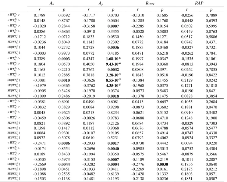
The correlation results can be seen in Table 4. In order to simplify this table, only the correlation results for A0, Ap, ROUT and the RAP index were included. The reason is that, for

A0 and Ap, the most significant correlations where found, while ROUT and the RAP index are

the parameters most linked to compliance. In this table, some statistically significant correlations between wavelet parameters and A0, Ap and ROUT can be found. The most significant correlations appeared for the correlations between <WTB₂> and Ap and for the

correlations between SD WT_B

2

!" #$ and Ap.

INSERT TABLE 4 AROUND HERE

4.

DISCUSSION

In this study, the changes produced in WT and WE during the phases of ITs in patients with hydrocephalus were analysed. Specifically, we have explored the changes in WT and WE during ITs in frequency bands B1 (0.15-0.3 Hz) and B2 (0.67-2.5 Hz), associated with the respiratory and the pulse components of the ICP waveform, respectively [25].

4.1. Dynamical properties of ICP recordings

found a significant increase in SD WT_B

1

E₂

!" #$ with respect to SD WT_B

1

E0

!" #$ and in SD WT_B

1

E₂

!" #$ with

respect to SD WT_B

1

E₃

!" #$. These findings suggest that there is a significantly higher variability in

the spectral content of band B1 when CSF pressure reaches the range of intracranial hypertension. In the case of band B2, we found significant differences between the basal phase and the remaining phases of the ITs using <WT_B

2 > and SD WT!" B2#$. It should be noted that

our results showed a significant increase in <WT_B

2

E₂ >

with respect to <WT_B

2

E0 >_{. This result}

suggests an increase in the average degree of similarity in the spectral content during the state of intracranial hypertension when compared with the resting state. However, these spectral changes appear only in B2, indicating that this similarity increase is mainly associated to the pulse waves [11]. Furthermore, <WT > can be considered as an indirect measure of signal irregularity [35]. In this sense, the aforementioned results suggest an irregularity loss in E2 with respect to E0. In previous studies, a decrease in Lempel-Ziv (LZ) complexity in the plateau phase of ITs with respect to the basal phase was reported [8]. Reduced complexity was also found in paediatric patients suffering from traumatic brain injury and intracranial hypertension [15]. Certainly, complexity and irregularity are complementary measures that quantify the degree of disorder in the different phases of ITs. It should also be stressed that a significant decrease in SD WTB₂

E2

!" #$ with respect to SD WT_B

2

E₀ !

" #$ was found. This result can be associated with a loss of variability in the plateau phase when compared with the basal phase.

Regarding WE, the differences between phases of the IT were not statistically significant for frequency band B1. However, results in Table 3 indicate that significant differences between the basal phase and the remaining phases of the IT could be detected in B2, using both < >

2

B

WE and SD WE!" B₂#$. Besides, we also found statistically significant differences

<WE_B

2

E2 > _{with respect to} <_WE

B₂ E_{0 >}

was detected. This result suggests that the spectral distribution in the hypertension state is less irregular than in the resting state [39]. These findings for band B2 are concordant with the results obtained with WT. As formerly stated, similar results were found using complexity measures in previous studies [8,15]. It should also be stressed that a significant decrease in SD WE_B

2

E₂

!" #$ with respect to SD WE_B

2

E₀

!" #$ was

found. These results suggest that intracranial hypertension due to volume loading produces a significantly lower variability in the spectral content of band B2. This variability decrease could be linked to the decrease in data dispersion found in previous studies on ITs, measured in terms of the standard deviation of LZ values [8]. In this study, the SD in LZ complexity values was lower in the plateau phase than in the basal phase. Oppositely, other studies reported an increased variability in the ICP signal during the plateau phase of ITs [40]. However, variability was measured in terms of data dispersion using central tendency measure (CTM). SD

[ ]

WE differs from CTM, since it quantifies temporal variability as the homogeneity in WE values along phases of the IT.

4.2. Respiratory and pulse-driven abnormalities in NPH

during diastole [41]. These blood volume changes during the cardiac cycle must be compensated by the CSF volume changes in order to maintain a stable ICP, leading to ABP-driven pulsations in CSF pressure [41]. However, vascular compliance seems to be reduced in disorders such as NPH [42]. Besides, it has been suggested that volume load during ITs may also have a relevant impact in the compliance of the brain and cerebral blood vessels. This issue leads to an exhausted compensatory reserve in the plateau phase of ITs, independently of the pathogenesis of hydrocephalus [7,43]. In this study, we found a decrease in irregularity and variability, together with a higher degree of similarity in the spectral content of the ICP waveform in the plateau phase with respect to the basal phase. These changes were mainly observed in band B2, related to pulse waves [25]. Therefore, they might be related to modifications in the ICP waveform associated with reduced brain compliance in NPH or with hypertension induced by ITs. Additional measures would be needed to confirm this relationship.

In this sense, it has been suggested that a reduced brain compliance may be associated with distinctive morphological patterns of the ICP pulse waves [21,44]. Therefore, the shape of ICP pulse waves may change during ITs, from patterns representing undistorted compliance to patterns representing reduced brain compliance. This shape change of pulse waves may be connected with the differences found in < >

2

B

WT , SD WT_B

2

!" #$, < >

2

B

WE and SD WE_B

2

!" #$,

especially when comparing E2 and E0.

Consequently, the arterial pulse pressure transmitted to the capillary circulation would be stronger [45]. In this study, we observed that the state of intracranial hypertension induced by ITs affects the ABP component of the ICP waveform (band B2), which is consistent with a disruption of the windkessel effect triggered by infusion.

Finally, some authors have suggested that elevated ICP may activate an intracranial baroreflex conducted through the autonomic system [47]. The moderate rise in ICP during ITs may result in a reversible pressure-driven systemic response. This produces an elevation in ABP and heart rate variance, as well as a decrease in cerebral perfusion pressure (CPP) and blood flow velocity (FV) [47]. The changes in ABP as a consequence of a moderate rise in ICP are compatible with an early Cushing response [47]. The differences in band B2 between E2 and E0 may reflect the influence of the moderate hypertension produced during ITs in systemic haemodynamics. Our results could be indicative of an adaptive haemodynamic response modulated by the presence of an intracranial baroreflex [47].

The statistically significant differences between phases of the IT were mainly found in B2, which leads us to hypothesise that the previous changes affect mainly the pulse component of the ICP waveform. However, some statistically significant differences were also observed in band B1, related to the respiratory-related component of the ICP waveform. Previous investigations also reported a relationship between pressure changes and the respiratory component of the ICP waveform [25,48]. It has been shown that, under reduced pressure-volume compliance conditions, ventilatory alternations in cerebral FV are reduced [25,48], while ICP appears to be unaffected [25]. Our results using SD WT_B

1

!" #$ suggest that there is a

experimental models [48] and evoked respiratory waves [25]. This may be the reason why our results show a weaker link between ICP and respiratory waves.

4.3. Relationship between wavelet parameters and patient data

We also analysed the correlation between wavelet parameters and several demographic, radiological and ICP-based variables extracted for the patients in our database. Results in Table 4 show that a few significant correlations could be found. The most significant correlations were related to the amplitude of the signal in the plateau phase (A_p). It is noteworthy that, in the case of < >

2

B

WT , significant correlations with A_pwere found in all

the artefact-free epochs of the infusion study. Besides, for SD WT!" B₂#$, significant correlations with A_pwere found for the basal, early infusion and recovery phases. These results suggest that the changes in the average degree of similarity in the spectral content and the variability of the ICP signal in band B2 are linked to changes in signal amplitude produced by intracranial hypertension induced by ITs.

4.4. Limitations of the study and future research lines

4.5. Conclusion

Wavelet parameters like WT and WE revealed changes in the signal time-scale representation during ITs. Our results show a higher degree of similarity in the spectral content of ICP signals, as well as a lower irregularity and variability in the plateau phase with respect to the basal phase in band B2. We also found statistically significant differences between E2 and E0 for band B1 using SD

[ ]

WT .

ACKNOWLEDGEMENTS

REFERENCES

[1] M. Bergsneider, C. Miller, Surgical management of adult hydrocephalus, Surgery. 62 (2008) 643–660.

[2] R.A. Weerakkody, M. Czosnyka, M.U. Schuhmann, E.A. Schmidt, N. Keong, T. Santarius, et al., Clinical assessment of cerebrospinal fluid dynamics in hydrocephalus. Guide to interpretation based on observational study, Acta Neurol. Scand. 124 (2011) 85–98.

[3] Y. Serulle, H. Rusinek, I.I. Kirov, H. Milch, E. Fieremans, A.B. Baxter, et al., Differentiating shunt-responsive normal pressure hydrocephalus from Alzheimer disease and normal aging: pilot study using automated MRI brain tissue segmentation., J. Neurol. 261 (2014) 1994–2002.

[4] A. Chari, M. Czosnyka, H.K. Richards, J.D. Pickard, Z.H. Czosnyka, Hydrocephalus shunt technology: 20 years of experience from the Cambridge Shunt Evaluation Laboratory., J. Neurosurg. 120 (2014) 697–707.

[5] N. Lenfeldt, A. Larsson, L. Nyberg, M. Andersson, R. Birgander, A. Eklund, et al., Idiopathic normal pressure hydrocephalus: increased supplementary motor activity accounts for improvement after CSF drainage., Brain. 131 (2008) 2904–12.

[6] P.K. Eide, Cardiac output in idiopathic normal pressure hydrocephalus: association with arterial blood pressure and intracranial pressure wave amplitudes and outcome of shunt surgery., Fluids Barriers CNS. 8 (2011) 11.

[7] M. Czosnyka, Z.H. Czosnyka, S. Momjian, J.D. Pickard, Cerebrospinal fluid dynamics., Physiol. Meas. 25 (2004) R51–R76.

[8] D. Santamarta, R. Hornero, D. Abásolo, M. Martínez-Madrigal, J. Fernández, J. García-Cosamalón, Complexity analysis of the cerebrospinal fluid pulse waveform during infusion studies, Child’s Nerv. Syst. 26 (2010) 1683–1689.

[9] A. Eklund, P. Smielewski, I. Chambers, N. Alperin, J. Malm, M. Czosnyka, et al., Assessment of cerebrospinal fluid outflow resistance, Med. Biol. Eng. Comput. 45 (2007) 719–735.

[10] A. Agren-Wilsson, A. Eklund, L.-O.D. Koskinen, A.T. Bergenheim, J. Malm, Brain energy metabolism and intracranial pressure in idiopathic adult hydrocephalus syndrome., J. Neurol. Neurosurg. Psychiatry. 76 (2005) 1088–1093.

[11] S. Momjian, Z.H. Czosnyka, M. Czosnyka, J.D. Pickard, Link between vasogenic waves of intracranial pressure and cerebrospinal fluid outflow resistance in normal pressure hydrocephalus., Br. J. Neurosurg. 18 (2004) 56–61.

[12] M. Czosnyka, J.D. Pickard, Monitoring and interpretation of intracranial pressure., J. Neurol. Neurosurg. Psychiatry. 75 (2004) 813–821.

[13] R. Hornero, M. Aboy, D. Abásolo, J. McNames, B. Goldstein, Interpretation of approximate entropy: Analysis of intracranial pressure approximate entropy during acute intracranial hypertension, IEEE Trans. Biomed. Eng. 52 (2005) 1671–1680. [14] C.-W. Lu, M. Czosnyka, J.-S. Shieh, A. Smielewska, J.D. Pickard, P. Smielewski,

injury., Brain. 135 (2012) 2399–408.

[15] R. Hornero, M. Aboy, D. Abásolo, Analysis of intracranial pressure during acute intracranial hypertension using Lempel-Ziv complexity: Further evidence, Med. Biol. Eng. Comput. 45 (2007) 617–620.

[16] J.J. Lemaire, J.Y. Boire, J. Chazal, B. Irthum, A computer software for frequential analysis of slow intracranial pressure waves, Comput. Methods Programs Biomed. 42 (1994) 1–14.

[17] S. Holm, P.K. Eide, The frequency domain versus time domain methods for processing of intracranial pressure (ICP) signals, Med. Eng. Phys. 30 (2008) 164–170.

[18] M. García, J. Poza, D. Santamarta, D. Abásolo, P. Barrio, R. Hornero, Spectral analysis of intracranial pressure signals recorded during infusion studies in patients with hydrocephalus., Med. Eng. Phys. 35 (2013) 1490–8.

[19] M. Kasprowicz, S. Asgari, M. Bergsneider, M. Czosnyka, R. Hamilton, X. Hu, Pattern recognition of overnight intracranial pressure slow waves using morphological features of intracranial pressure pulse, J. Neurosci. Methods. 190 (2010) 310–318.

[20] X. Hu, P. Xu, F. Scalzo, P. Vespa, M. Bergsneider, Morphological Clustering and Analysis of Continuous Intracranial Pressure, IEEE Trans. Biomed. Eng. 56 (2009) 696–705.

[21] I.M. Elixmann, M. Kwiecien, C. Goffin, M. Walter, B. Misgeld, M. Kiefer, et al., Control of an electromechanical hydrocephalus shunt--a new approach., IEEE Trans. Biomed. Eng. 61 (2014) 2379–88.

[22] M. Latka, W. Kolodziej, M. Turalska, D. Latka, W. Zub, B.J. West, Wavelet assessment of cerebrospinal compensatory reserve and cerebrovascular reactivity., Physiol. Meas. 28 (2007) 465–479.

[23] H.E. Heissler, K. König, J.K. Krauss, E. Rickels, Stationarity in Neuromonitoring Data, Acta Neurochir. Suppl. 114 (2012) 93–95.

[24] P. Xu, X. Hu, D. Yao, Improved wavelet entropy calculation with window functions and its preliminary application to study intracranial pressure, Comput. Biol. Med. 43 (2013) 425–433.

[25] C. Haubrich, R.R. Diehl, M. Kasprowicz, J. Diedler, E. Sorrentino, P. Smielewski, et al., Traumatic brain injury: Increasing ICP attenuates respiratory modulations of cerebral blood flow velocity, Med. Eng. Phys. 37 (2015) 175–179.

[26] O. Rioul, M. Vetterli, Wavelets and signal processing, IEEE Signal Process. Mag. 8 (1991) 14–38.

[27] C. Torrence, G.P. Compo, A Practical Guide to Wavelet Analysis, Bull. Am. Meteorol. Soc. 79 (1998) 61–78.

[28] S. Mallat, A Wavelet Tour of Signal Processing: The Sparse Way, Academic Press, 2008.

[29] B.J. Roach, D.H. Mathalon, Event-related EEG time-frequency analysis: An overview of measures and an analysis of early gamma band phase locking in schizophrenia, Schizophr. Bull. 34 (2008) 907–926.

study of event-related coupling patterns during an auditory oddball task in schizophrenia., J. Neural Eng. 12 (2015) 016007.

[31] J. Poza, C. Gómez, M. García, R. Corralejo, A. Fernández, R. Hornero, Analysis of neural dynamics in mild cognitive impairment and Alzheimer’s disease using wavelet turbulence., J. Neural Eng. 11 (2014) 026010.

[32] M. Turalska, M. Latka, K. Pierzchala, B.J. West, M. Czosnyka, Generation of very low frequency cerebral blood flow fluctuations in humans, Acta Neurochir. Suppl. 102 (2008) 43–47.

[33] P.R.B. Benchimol-Barbosa, A. de Souza-Bomfim, E. Corrêa-Barbosa, P. Ginefra, S.H. Cardoso-Boghossian, C. Destro, et al., Spectral turbulence analysis of the signal-averaged electrocardiogram of the atrial activation as predictor of recurrence of idiopathic and persistent atrial fibrillation, Int. J. Cardiol. 107 (2006) 307–316.

[34] J.W. Sleigh, D.A. Steyn-Ross, M.L. Steyn-Ross, C. Grant, G. Ludbrook, Cortical entropy changes with general anaesthesia: theory and experiment, Physiol. Meas. 25 (2004) 921–934.

[35] M. García, J. Poza, D. Abásolo, D. Santamarta, R. Hornero, Analysis of intracranial pressure signals recorded during infusion studies using the spectral entropy., in: Proc. Annu. Int. Conf. IEEE Eng. Med. Biol. Soc., 2013: pp. 2543–6.

[36] J.D. Jobson, Applied Multivariate Data Analysis, Springer New York, New York, NY, 1991.

[37] D.J. Kim, Z. Czosnyka, N. Keong, D.K. Radolovich, P. Smielewski, M.P.F. Sutcliffe, et al., Index of cerebrospinal compensatory reserve in hydrocephalus, Neurosurgery. 64 (2009) 494–502.

[38] M. Aboy, J. McNames, W. Wakeland, B. Goldstein, Pulse and mean intracranial pressure analysis in pediatric traumatic brain injury, in: Intracranial Press. Brain Monit. XII, Springer-Verlag, Vienna, 2005: pp. 307–310.

[39] J. Poza, R. Hornero, D. Abásolo, A. Fernández, M. García, Extraction of spectral based measures from MEG background oscillations in Alzheimer’s disease, Med. Eng. Phys. 29 (2007) 1073–1083.

[40] D. Santamarta, D. Abásolo, M. Martínez-Madrigal, R. Hornero, Characterisation of the intracranial pressure waveform during infusion studies by means of central tendency measure, Acta Neurochir. (Wien). 154 (2012) 1595–1602.

[41] G.A. Bateman, Vascular compliance in normal pressure hydrocephalus, Am. J. Neuroradiol. 21 (2000) 1574–1585.

[42] M.E. Wagshul, E.J. Kelly, H.J. Yu, B. Garlick, T. Zimmerman, M.R. Egnor, Resonant and notch behavior in intracranial pressure dynamics, J. Neurosurg. Pediatr. 3 (2009) 354–364.

[43] C. Haubrich, Z.H. Czosnyka, A. Lavinio, P. Smielewski, R.R. Diehl, J.D. Pickard, et al., Is there a direct link between cerebrovascular activity and cerebrospinal fluid pressure-volume compensation?, Stroke. 38 (2007) 2677–2680.

communicating hydrocephalus, Pediatr. Neurosurg. 36 (2002) 281–303.

[46] G.A. Bateman, C.R. Levi, P. Schofield, Y. Wang, E.C. Lovett, The venous manifestations of pulse wave encephalopathy: windkessel dysfunction in normal aging and senile dementia., Neuroradiology. 50 (2008) 491–7.

[47] E.A. Schmidt, Z.H. Czosnyka, S. Momjian, M. Czosnyka, R.A. Bech, J.D. Pickard, Intracranial baroreflex yielding an early Cushing response in human, Acta Neurochir. Suppl. 95 (2005) 253–256.

[48] X. Hu, A.A. Alwan, E.H. Rubinstein, M. Bergsneider, Reduction of compartment compliance increases venous flow pulsatility and lowers apparent vascular compliance: implications for cerebral blood flow hemodynamics., Med. Eng. Phys. 28 (2006) 304– 14.

TABLES

Table 1. Data recorded from the subjects under study.

Table 2. Median [interquartile range, IQR] values of the epoch length and CSF pressure.

Table 3. Z statistics and p-values associated with the Wilcoxon signed-rank tests. The significant values (p<1.70×10-3, Bonferroni-corrected) are highlighted.

FIGURE LEGENDS

Figure 1. Evolution of the CSF pressure during the infusion test for a patient diagnosed with normal pressure hydrocephalus. The four artefact-free epochs selected by a neurosurgeon have been indicated (E0: epoch 0, E1: epoch 1, E2: epoch 2, E3: epoch 3).

Figure 2. Scalogram obtained for the ICP recording of Fig. 1. The transparency outline delineates the limits of the cone of influence (COI), where border effects can be ignored. The black horizontal lines indicate the limits of frequency bands B1 (0.15 - 0.3 Hz) and B2 (0.67 – 2.5 Hz).

Figure 3. Boxplots displaying the distribution of <WT> and SD[WT] for frequency bands B1

and B2 in the four artefact-free epochs. (a) <WTB₁>. (b) SD WT!" B₁#$. (c) <WTB₂ >. (d)

SD WT_B

2

!" #$. The statistically significant differences are indicated with an asterisk

(* 3

10 70 .

1 ×

-<

p , Bonferroni-corrected).

Figure 4. Boxplots displaying the distribution of <WE> and SD[WE] for frequency bands B1

and B2 in the four artefact-free epochs. (a) < >

1

B

WE . (b) SD WE!" B₁#$. (c) <WEB₂ >. (d)

SD WE_B

2

!" #$. The statistically significant differences are indicated with an asterisk

(*p<1.70×10-3, Bonferroni-corrected).

Table 1. Data recorded from the subjects under study.

IQR: interquartile range

Characteristic Value

(median [IQR])

Number of subjects (n) 112

Age (years) 74 [63-80]

Ventricular size (Evans index, E) 0.37 [0.35-0.41]

Basal pressure (P₀) (mm Hg) 7.71 [5.53-11.10]

Basal amplitude (A₀) (mm Hg) 2.73 [1.57-3.46]

Plateau pressure (P_p) (mm Hg) 24.95 [18.57-32.67]

Plateau amplitude (A_p) (mm Hg) 9.74 [5.93-13.85]

Table 2. Median [interquartile range, IQR] values of the epoch length and CSF pressure.

CSF: cerebrospinal fluid

Epoch 0 Epoch 1 Epoch 2 Epoch 3

Length (s) 156 [120-180] 300 [240-330] 480 [360-600] 180 [130-205] CSF pressure

Table 3. Z statistics and p-values associated with the Wilcoxon signed-rank tests. The significant values (p1.70103, Bonferroni-corrected) are highlighted.

E0 vs. E1 E0 vs. E2 E0 vs. E3 E1 vs. E2 E1 vs. E3 E2 vs. E3

Z p Z p Z p Z p Z p Z p



WTB₁ -2.85 4.40·10-3 -2.97 3.01·10-3 -1.66 9.68·10-2 -2.42 1.55·10-2 -0.50 0.62 -2.73 6.24·10-3

] SD[

1

B

WT -2.65 7.83·10-3 _{-3.19 1.43·10}-3 _{-1.31 0.19 -1.59 0.11 -2.08 3.79·10}-2 _{-3.38 7.35·10}-4



WTB₂ -6.13 8.71·10-10 -7.80 6.16·10-15 -1.42 1.14·10-13 -3.06 2.21·10-3 -0.38 0.71 -2.85 4.44·10-3

] SD[

2

B

WT -5.82 5.86·10-9 _{-6.90 5.17·10}-12 _{-7.04 1.96·10}-12 _{-1.63 0.10 -1.17 0.24 -0.61 0.54}



WEB₁ -1.66 9.68·10-2 -2.97 2.98·10-3 -2.41 1.61·10-2 -1.72 8.57·10-2 -2.23 2.56·10-2 -0.18 0.86



WEB₂ -6.05 1.45·10-9 -6.15 7.95·10-10 -5.40 6.56·10-8 -1.80 7.19·10-2 -1.08 0.28 -2.94 3.27·10-3

] SD[

2

B

WE -6.77 1.29·10-11 _{-7.30 2.91·10}-13 _{-7.49 6.88·10}-14 _{-5.48 4.30·10}-8 _{-4.02 5.87·10}-5 _{-1.70 8.95·10}-2

E0: epoch 0; E1: epoch 1; E2: epoch 2; E3: epoch 3;  

1

B

WT : mean wavelet turbulence in band B₁; SD[ ]

1

B

WT : standard deviation of the wavelet turbulence in band B₁;  

2

B

WT : mean wavelet turbulence in band B₂; SD[ ]

2

B

WT : standard deviation of the wavelet turbulence in band B₂;  

1

B

WE : mean wavelet entropy in band B₁;  

2

B

WE : mean wavelet entropy in band B₂;

] [

Table 4.-. Correlation coefficients, r, and p-values obtained for the Spearman test to determine correlation between wavelet parameters and patient data. Values with a significance level p0.01 are highlighted.

A0 Ap ROUT RAP

r p r p r p r p

  0

1

E B

WT _{0.1789 0.0592 -0.1717 0.0703 -0.1310 0.1685 -0,0256 0,7889}

  1

1

E B

WT _{0.0148 0.8767 -0.1780 0.0604 -0.1285 0.1768 -0,0448 0,6393}

  2

1

E B

WT _{-0.1020 0.2844 -0.3158 0.0007 -0.2285 0.0154 0,0502 0,5995}

  3

1

E B

WT _{0.0386 0.6863 -0.0918 0.3355 -0.0528 0.5803 0,0149 0,8763}

] SD[ 0

1

E B

WT _{-0.1712 0.0712 0.1833 0.0530 0.1450 0.1271 0,0517 0,5886}

] SD[ 1

1

E B

WT _{-0.0236 0.8049 0.1143 0.2302 0.0772 0.4184 0,0742 0,4371}

] SD[ 2

1

E B

WT _{0.1044 0.2732 0.2728 0.0036 0.1883 0.0468 -0,0327 0,7321}

] SD[ 3

1

E B

WT _{-0.0003 0.9973 0.0772 0.4185 0.0471 0.6218 -0,0262 0,7841} 

 0 2

E B

WT _{0.3389 0.0003 0.4347 1.68}₁₀-6 _{0.1997 0.0347 -0,1535 0,1061}

  1

2

E B

WT _{0.1804 0.0570 0.4050 9.43}₁₀-6 _{0.1984 0.0360 -0,0813 0,3943}

  2

2

E B

WT _{0.1165 0.2210 0.2762 0.0032 0.0808 0.3971 0,0262 0,7835}

  3

2

E B

WT _{0.1012 0.2885 0.3818 3.28}₁₀-5 _{0.1843 0.0518 -0,0190 0,8422}

] SD[ 0

2

E B

WT _{-0.3081 0.0010 -0.3626 8.55}₁₀-5 _{-0.1384 0.1455 0,2129 0,0242}

] SD[ 1

2

E B

WT -0.1979 0.0365 -0.3762 4.3510-5 _{-0.1968 0.0375 0,1271 0,1818}

] SD[ 2

2

E B

WT _{-0.0905 0.3426 -0.1970 0.0374 -0.0573 0.5483 -0,0190 0,8421}

] SD[ 3

2

E B

WT _{-0.1099 0.2486 -0.2919 0.0018 -0.1378 0.1475 0,0828 0,3854} 

 0 1

E B

WE _{-0.0381 0.6901 0.0490 0.6081 0.0413 0.6657 0,1055 0,2684}

  1

1

E B

WE _{-0.0832 0.3829 0.0084 0.9298 -0.0873 0.3602 0,1881 0,0470}

  2

1

E B

WE _{0.0045 0.9625 0.0213 0.8234 -0.0621 0.5152 0,0910 0,3402}

  3

1

E B

WE _{-0.0459 0.6306 -0.0026 0.9783 -0.0688 0.4710 0,1248 0,1900}

] SD[ 0

1

E B

WE _{0.0821 0.3892 0.1187 0.2126 0.0684 0.4734 -0,0329 0,7303}

] SD[ 1

1

E B

WE _{0.1398 0.1417 0.0112 0.9068 0.0676 0.4788 -0,0574 0,5477}

] SD[ 2

1

E B

WE _{0.0084 0.9301 -0.0107 0.9105 0.0657 0.4914 -0,0747 0,4338}

] SD[ 3

1

E B

WE 0.0972 0.3078 0.0610 0.5231 0.0792 0.4062 -0,0924 0,3327 

 0 2

E B

WE _{-0.2471 0.0086 -0.2933 0.0017 -0.0730 0.4442 0,0094 0,9220}

  1

2

E B

WE _{-0.0174 0.8554 -0.2696 0.0040 -0.0985 0.3013 -0,0752 0,4304}

  2

2

E B

WE _{0.0189 0.8430 -0.1994 0.0350 -0.0575 0.5467 -0,0879 0,3566}

  3

2

E B

WE _{-0.0505 0.5973 -0.3153 0.0007 -0.1189 0.2119 -0,1011 0,2887}

] SD[ 0

2

E B

WE -0.2669 0.0044 -0.3282 0.0004 -0.2776 0.0030 0,1756 0,0640

] SD[ 1

2

E B

WE -0.1898 0.0451 -0.1933 0.0411 -0.2269 0.0161 0,2175 0,0212

] SD[ 2

2

E B

WE _{-0.1088 0.2535 -0.0482 0.6139 -0.1428 0.1332 0,1803 0,0571}

] SD[ 3

2

E B