COMPREHENSIVE ANALYSIS OF PREBIOTIC PROPENAL UP TO 660 GHz
A. M. Daly1,2, C. Bermúdez1, L. Kolesniková1, and J. L. Alonso1 1
Grupo de Espectroscopia Molecular(GEM), Edificio Quifima, Área de Química-Física, Laboratorios de Espectroscopia y Bioespectroscopia, Parque Científico UVa, Unidad Asociada CSIC, Universidad de Valladolid, E-47011 Valladolid, Spain;[email protected]
2
Jet Propulsion Laboratory, California Institute of Technology, 4800 Oak Grove Dr., Pasadena, CA 91109, USA
Received 2015 March 13; accepted 2015 May 8; published 2015 June 22
ABSTRACT
Since interstellar detection of propenal is only based on two rotational transitions in the centimeter wave region, its high resolution rotational spectrum has been measured up to 660 GHz and fully characterized by assignment of more than 12,000 transitions to provide direct laboratory data to the astronomical community. Spectral assignments and analysis include transitions from the ground state of thetransandcisisomers, threetrans-13C isotopologues, and ten excited vibrational states of thetransform. Combining new millimeter and submillimeter data with those from the far-infrared region has yielded the most precise set of spectroscopic constants oftrans-propenal obtained to date. Newly determined rotational constants, centrifugal distortion constants, vibrational energies, and Coriolis and Fermi interaction constants are given with high accuracy and were used to predict transition frequencies and intensities over a wide frequency range. Results of this work should facilitate astronomers further observation of propenal in the interstellar medium.
Key words:catalogs –ISM: molecules –molecular data–techniques: spectroscopic
Supporting material:machine-readable tables
1. INTRODUCTION
Ever since the discovery of the simplest aldehyde ( for-maldehyde)in the interstellar medium (ISM), aldehydes have also been called the “sugars of space” (Snyder et al. 1969). Detection of these “sugars of space” is associated mainly to molecular clouds, which may indicate that the reactions occuring in grains facilitate their formation (Ikeda et al. 2001). So far, the observation of lines belonging to these aldehydes is restricted to molecules with chains contain-ing no more than three carbon atoms, with propenal(acrolein), CH2CHCHO, the simplest conjugated aldehyde, being one of the largest. Additionally, propenal is considered to be a prebiotic molecule owing both to its formation in the decomposition of sugars (Moldoveanu 2010; Bermúdez et al. 2013) and its implication in the synthesis of amino acids, such as methionine and glutamic acid, via Strecker-type reactions(van Trump & Miller1972). Its generation in the ISM has been postulated to be a product of a simple hydrogen addition reaction from a known interstellar aldehyde, propynal
(Irvine et al. 1988; Turner 1991). Nevertheless, while more than 40 transitions have been found belonging to other relevant aldehydes, such as glycoladehyde, in different regions of the ISM(Hollis et al.2000; Halfen et al.2006; Beltrán et al.2009; Jørgensen et al.2012), positive detection of propenal has thus far been based on only two transitions of its lower energytrans isomer in the ground vibrational state, namely 211¬110 and the 313 ¬212 at 18221.164 (2) and 26079.449 (1)MHz, respectively, observed by the 100 m Green Bank Telescope pointing toward the star-forming region of Sagittarius B2(N)
(Hollis et al. 2004; Requena-Torres et al. 2008). With the increasing sensitivity of astrophysical detection facilities, it might now be possible to identify not only further lines of trans-propenal, but also transitions from 13C isotopologues, excited vibrational states, or the higher energy cis isomeric form. The key to success in this astrophysical identification lies in analyzing propenal pure rotational transitions, especially those that fall into the millimeter- and submillimeter-wave
regions, which are the working domains for the IRAM, NRAO, SEST, CSO telescopes, or ALMA interferometers.
Propenal can be observed in two trans and cis planar Cs conformers that interchange by rotation around the single C–C bond(seefigures in Table1), thecisform being 600 cm−1 higher in energy than the trans one (Blom & Bauder 1982). Ground state rotational spectra of both conformers, their isotopologues, and the lowest-energy excited vibrational state have already been studied in the microwave region (Fine et al. 1955; Wagner et al. 1957; Cherniak & Costain 1966; Blom & Bauder1982; Blom et al.1984). However, apart from the ground vibrational state oftrans-propenal, which has been analyzed up to 170 GHz(Winnewisser et al.1975), no further information exists on the rotational spectrum of propenal. Since there is always an uncertainty involved in predicting transitions at higher frequencies, interstellar detection of new propenal lines should be based on transitions measured directly in the laboratory or transitions predicted from a data set that includes higher frequency lines. In the present work, the pure rotational spectrum of propenal up to 660 GHz has been analyzed for the ground vibrational state of cis- and trans-propenal, the three 13
C isotopologues of the latter and ten lowest energy excited vibrational states below 700 cm−1. Given the strong Coriolis and Fermi perturbations observed, a global fit analysis combining our pure rotational and previously published vibrational rotational data(McKellar et al.2007; McKellar & Appadoo 2008) was required. A highly accurate set of spectroscopic parameters that reproduce the spectrum and can facilitate detections of propenal in the ISM was thus obtained.
2. EXPERIMENTAL DETAILS
A commercially available sample of liquid propenal
(b.p.=125°C)was used without further purification. Propenal spectrum was acquired using two different spectrometers. A recently upgraded Stark-modulation spectrometer employing 33 kHz modulation frequency and phase-sensitive detection
26–110 GHz range. Millimeter- and submillimeter-wave mea-surements, over the 50–660 GHz range, were performed using a direct absorption spectrometer recently constructed at the University of Valladolid (Daly et al.2014). It is based on the frequency multiplier chains (VDI, Inc.) driven by an Agilent E8257D microwave synthesizer. The signal was detected using solid-state zero-bias detectors (VDI, Inc.) at twice the modulation frequency (2f =20.4 kHz)and with a modulation depth between 20 and 50 kHz resulting in the second derivative line shape. All spectra were taken at room temperature with sample pressure less than 30 mTorr and recorded in 1 GHz sections in both directions. Rotational spectra of all three 13C isotopologues were measured in their natural abundances. Transition lines were measured using a Gaussian profile function (AABS package; Kisiel et al. 2005) with accuracy better than 50 kHz for isolated well-developed lines (the accuracy up to 500 kHz was given to lines with poor signal-to-noise ratio).
3. ROTATIONAL SPECTRA AND ANALYSIS
3.1. Ground Vibrational State
The ground state rotational spectrum of trans-propenal is dominated by stronga-typeR-branch transitions and weakerb -typeR-branch andQ-branch transitions, in agreement with the values of the dipole moment components∣ ∣ma = 3.052(4)D and∣mb∣ = 0.630(1)D(Blom et al.1984). Starting with the predictions based on the previous results and following an iterative process of assignment andfitting, over 1900 lines were
assigned up toJ=76 andKa=24. The following WatsonʼsA -reduced semi-rigid Hamiltonian up to the sixth order
(Watson1977)was used in the analysis
d d
f f
f
= + + - D - D
- D - éëê + + ùûú
+ F + F + F
+ F + éëê +
+ + ùûú
+ - +
+ - +
H AJ BJ CJ J J J
J J J J J
J J J J J
J J J J
J J J
1
2 ,
1 2
, (1)
v
a b c J JK a
K a J K a
J JK a KJ a
K a J JK a
K a
Rot
( ) 2 2 2 4 2 2
4 2 2 2 2
6 4 2 2 4
6 4 2 2
4 2 2
whereA,B,Care the rotational constants,ΔJ,ΔJK,ΔK,δJ,δK are quartic, and ΦJ, ΦJK, ΦKJ, ΦK, ϕJ, ϕJK, ϕK are sextic centrifugal distortion constants. Some series of high Ka -rotational transitions were found to be perturbed and could not be fitted within the distortable rotor model, hence, they were not included in the current stage of the fit. These perturbations were later treated in the global analysis presented in the following section. The spectroscopic parameters derived are listed in thefirst column of Table1.
Around 500 distinct frequency ground state lines for each 13C-species were analyzed in terms of the same Hamiltonian
given by Equation(1)withΦJK,ϕJ, andϕJKconstantsfixed to the values of the parent species. Since our measurements were performed in natural abundance (intensities about 1% of the parent species), only the intense a-type transitions were
Table 1
Ground State Spectroscopic Constants of theTrans-propenal Parent and13C-species andCis-propenal(A-reduction,Ir-representation)
Constant Unit Trans-propenal Trans-13C1 Trans
-13
C2 Trans -13
C3 Cis-propenal
L L
A MHz 47353.7074(17)a 46781.0275(67) 46518.9165(64) 47255.1934(73) 22831.6487(43)
B MHz 4659.499468(61) 4644.74135(19) 4642.43842(17) 4520.79374(15) 6241.04728(35)
C MHz 4242.689488(56) 4225.83534(20) 4221.74338(19) 4126.64084(18) 4902.20757(21)
ΔJ kHz 1.042067(19) 1.03970(10) 1.03172(10) 0.988410(65) 5.11335(24)
ΔJK kHz −8.78538(44) −8.6890(24) −8.7575(13) −8.9704(14) −29.1854(13)
ΔK kHz 360.363(64) 348.56(23) 367.21(22) 363.31(26) 108.07(12)
δJ kHz 0.1202675(76) 0.120817(20) 0.121459(18) 0.111595(18) 1.48116(12)
δK kHz 5.7481(24) 5.643(10) 5.745(10) 5.441(10) 11.3386(76)
ΦJb
mHz 0.2994(25) 0.209(20) 0.274(21) 0.287(11) 1.601(89)
ΦJK mHz −6.576(46) −6.576c −6.576c −6.576c 92.04(49)
ΦKJ mHz −510.0(12) −382(19) −536.1(64) −459.1(70) −1153.0(21)
ϕJ mHz 0.0740(11) 0.0740c 0.0740c 0.0740c 1.082(43)
ϕJK mHz 5.00(62) 5.00c 5.00c 5.00c −19.3(20)
Jrange L 5−73 1−55 1−55 1−67 1−61
Karange L 0−19 0−12 0−16 0−16 0−23
Nlines/Nexd L 1606/28 492/103 531/85 485/93 574/78
σfite kHz 37 40 40 41 39
Note.
a
The numbers in parentheses are 1σuncertainties in the units of the last decimal digit. b
PurelyK-dependent sextic centrifugal distortion constantsΦKandϕKcould not be determined from the present data sets.
c
Fixed to the parent species value. d
Number of distinct frequencyfitted lines/number of excluded lines based on the 2ufitting criterion of the SPFIT program(Pickett1991)whereuis the uncertainty of the measured frequency. The uncertainties between 50 and 500 kHz were given to the millimeter and submillimeter data from this work and 100 kHz to the microwave data from Blom & Bauder(1982), Blom et al.(1984).
e
observed. These transitions were combined with thea- and b -type ones measured by Blom et al. (1984)using isotopically highly enriched samples. The final sets of the spectroscopic constants are also given in Table1.
Forcis-propenal(∣ ∣ma =2.010(5)D and∣mb∣=1.573(3)D
(Blom & Bauder1982)), more than 500 lines were assigned to a- andb-typeR-branch transitions up to J=60 andKa=23 and were analyzed using the above-mentioned Hamiltonian. The derived spectroscopic constants are listed in the last column of Table 1. Line assignments, observed frequencies νobs,νobs−νcalcvalues, whereνcalcis the calculated frequency based on the Hamiltonian model used, and references of the data sources included in thefinalfits for thetrans-13C-species and cis-propenal ground states are presented in Table2.
3.2. Excited Vibrational States
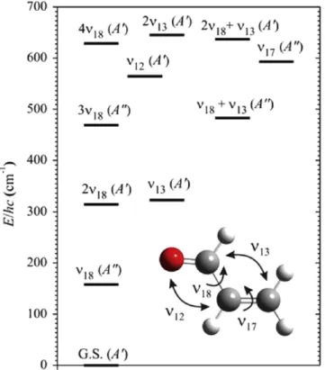
Trans-propenal has four low-lying vibrational modes invol-ving skeletal C–C torsion (ν18), C=C–C bending (ν13), O=C–C bending(ν12), and=CH2twisting mode(ν17). Up to 10 vibrational states below 700 cm−1 (see Figure 1) can be sufficiently populated at the room temperature of the experi-ment to generate a highly rich vibrational satellite spectrum. Stark-modulation microwave spectroscopy is a very useful tool for analyzing these rotational satellite lines as has recently been shown in works on ethyl(Daly et al.2014)and vinyl cyanide
(López et al. 2014). When an electric field is applied to a rotating molecule, the M-degeneracy is partially or fully removed. This perturbation of the rotational energy levels by electric field gives rise to a Stark spectrum. A section of the Stark spectrum around the ground state 414 ¬313 rotational transition oftrans-propenal is presented in Figure2. Rotational transitions in the excited vibrational states were readily
assigned on the basis of their characteristic Stark patterns
(negative lobes in Figure2), the same as the ground state line. Hence, at the higher frequency side of the ground state line, a harmonic progression formed by four satellite lines can easily be identified and assigned to pure rotational transition in successive excited vibrational states of thev18torsional mode. Moreover, pure rotational spectra in other excited states corresponding to v13 = 1, v12 = 1, v17 = 1 as well as combination states(v18=1,v13=1)and(v18=2,v13 =1) were also observed. Preliminary spectroscopic constants obtained for these 10 excited states were used to predict the corresponding rotational spectra in the millimeter- and submillimeter-wave region. Loomis–Wood type plots, origin-ally described by Loomis & Wood (1928), from the AABS package (Kisiel et al. 2005, 2012) were used to facilitate identification of rotational transitions for each vibrational state. During the analysis of propenal in the millimeter and submillimeter region, the major complication is due to the mutual interactions between excited vibrational states belong-ing to low-lybelong-ing vibrational modes leadbelong-ing to strong perturba-tions in the spectrum. The possible interacperturba-tions between two states depends on the symmetry classification of the states involved which is marked in Figure 1 according to the Cs symmetry point group. Vibrational states belonging to different symmetry species may be connected bya- andb-type Coriolis interaction terms, and excited states with the same symmetry species may be coupled through c-type Coriolis and Fermi interactions. Figure 1 shows how the lowest-energy v18 = 1 excited state should be free of interactions due to its energy spacing with respect to other excited states. Over 1000 pure rotational transitions could be included in the fit using the Equation (1). Nonetheless, several Ka series revealed devia-tions that could not be taken into account by adding
higher-Table 2
Laboratory Assigned and Fitted Transition Frequencies for theTrans-propenal Parent,Trans-13C-species,Cis-propenal Ground States and
Ten Excited Vibrational States ofTrans-propenal
Transitiona νobs
b
νobs−νcalc c
Species J′ Ka¢ Kc¢ v′ J″ Ka Kc v″ (MHz/cm
−1) (MHz/cm−1) Commentd
References
Trans-13C
1 16 1 16 0 15 1 15 0 138100.896 0.040 L (2)
Trans-13C
1 16 0 16 0 15 0 15 0 139964.297 0.020 L (2)
Trans-13C
2 20 7 13 0 19 7 12 0 177365.923 −0.031 L (2)
Trans-13C
2 20 6 14 0 19 6 13 0 177394.047 0.053 B (2)
Trans-13C
2 20 6 15 0 19 6 14 0 177394.047 0.056 B (2)
Trans-13C
3 16 0 16 0 15 0 15 0 136624.069 0.005 L (2)
Trans-13C
3 20 1 19 0 19 1 18 0 175805.698 0.121 U (2)
Cis 17 1 16 0 16 1 15 0 182121.954 −0.030 L (2)
Cis 16 2 14 0 15 2 13 0 184240.673 −0.006 L (2)
Trans 23 2 22 0 22 2 21 0 203709.166 −0.031 L (2)
Trans 23 2 22 3 22 2 21 3 203716.290 0.012 L (2)
Trans 23 2 22 10 22 2 21 10 203840.124 −0.005 L (2)
Notes. a
Upper and lower state quantum numbers are indicated by“and,”respectively. The assignment of the individual vibrational states tovis as following: 0ground state, 1v18=1, 2v18=2, 3v13=1, 4v18=3, 5(v18=1,v13=1), 6v12=1, 7v17=1, 8v18=4, 9(v18=2,v13=1), and
10v13=2.
b
Observed frequency. Microwave, millimeter and submillimeter data are in MHz while the far-infrared data are in cm−1. c
Observed minus calculated frequency. d
Blended transitions werefitted to their intensity weighted averages and are labeled by B. Unfitted transitions are labeled by U.
References.(1)Blom et al.(1984);(2)This work;(3)Blom & Bauder(1982);(4)Winnewisser et al.(1975);(5)McKellar & Appadoo(2008).
order centrifugal distortion effects. Some of these anomalies were observed exactly within the same range of theJquantum numbers as those already observed for ground state transitions. This clearly indicates that the ground state is in mutual interaction with thev18=1 excited state and, as a result, they were analyzed together. Even though both a- and b-type Coriolis couplings are allowed in this case, onlyb-type Coriolis terms were found to be significant in thefitting. Including the Coriolis terms in the analysis improved the fit considerably, although, several Kaseries of transitions inv18=1 could still not be reproduced. A deeper insight into thev18=1 rotational energy levels showed further interactions with higher-energy v18=2 state. This significantly complicates the analysis since the v18 =2 state cannot be analyzed without the neighboring
almost iso-energeticv13=1 state due to strongc-type Coriolis and Fermi interactions between them. A close look at the microwave spectrum in Figure 2 shows a small shift of the v18 = 2 transition from the equidistant pattern which reflects the strong coupling between this state andv13=1. A 4-state Hamiltonian analysis was thus performed to correctly repro-duce all the perturbed transitions in the ground state,v18=1, v18 =2, andv13 = 1 excited vibrational states. Two excited vibrational states,v18=3 and (v18=1, v13=1), were then also analyzed as an interacting pair connected through c-type Coriolis and Fermi interactions. Possible interactions of this pair with other states were ignored. Analysis of the five remaining excited vibrational states above 500 cm−1led to the identification of many local perturbations. Although thev12=1 and v17 = 1 pair was initially treated separately, a 5-state Hamiltonian including v12 =1, v17 = 1, v18 = 4, (v18 =2, v13=1), andv13=2 excited vibrational states was inevitable.
3.3. Global Analysis
Over 10,000 distinct frequency lines treated in the above-mentioned 4-state, 2-state, and 5-state analyses were finally combined with more than 8000 lines available from high resolution vibration-rotation study of McKellar & Appadoo
(2008). The uncertainties between 50 and 500 kHz were given to the millimeter and submillimeter data and between 0.0003 and 0.001 cm−1to the far-infrared data for weighing purposes of the nonlinear least-square fit. The Hamiltonian matrix constructed for this problem can be written in standard block form with 11 × 11 array size. Each diagonal block consists of
+ D
HRot( )v Ev term where HRotv
( ) is the Watsonʼs A-reduced rotational Hamiltonian for given vibrational statevdefined by Equation (1) and ΔEv = Ev − E0 is the vibrational energy difference from the ground state. The vibrational identifiers v are assigned to individual vibrational states as follows: 0ground state, 1v18 =1, 2v18=2, 3v13 =1, 4 v18=3, 5(v18=1,v13=1), 6v12=1, 7v17=1, 8 v18=4, 9(v18=2,v13=1), and 10v13=2. The off-diagonal blocks are composed by the Coriolis and Fermi interaction Hamiltonians aHCor( , )v v¢ and HF( , )v v¢, respectively, and were used when clear evidence of the mutual interactions between two statesvandv′was found. The leading terms of the α-type Coriolis Hamiltonian up to the second power in angular
Figure 1.Vibrational energy levels oftrans-propenal below 700 cm−1obtained by McKellar & Appadoo(2008)and schematic illustration of the four lowest-energy normal vibrational modes, ν18: C–C torsion, ν13: C=C–C bending
mode, ν12: O=C–C bending mode, and ν17: =CH2 twisting mode. The
symmetry specifications are given in accordance withCspoint group.
momentum are (Prevalov & Tyuterev1982)
= + +
a
a a bg b g g b
¢
(
)
HCor( , )v v iG J F J J J J (2)
whereGαand Fβγare the Coriolis coupling constantsα,β,γ are the permutations of a, b, c. The Fermi interaction
Hamiltonian up to the second power in angular momentum is given as(Prevalov & Tyuterev1982)
= + + +
-¢
(
)
HF( , )v v W W JJ 2 W JK a2 W Jb2 Jc2 (3)
Table 3
Spectroscopic Constants ofTrans-propenal for Each Vibrational Statevincluded in the Global 11-state Fit(A-reduction,Ir-representation)
va
OCb Constantc Unit 0 1 2 3 4 5
100vv′ A MHz 47353.6999(17)d 45782.9630(50) 44374.617(61) 48755.457(49) 43101.272(93) 46956.217(86) 200vv′ B MHz 4659.499451(93) 4666.24463(33) 4672.9124(10) 4659.3132(10) 4679.4475(17) 4665.4082(17) 300vv′ C MHz 4242.689513(86) 4259.62456(32) 4276.62153(90) 4238.35294(96) 4293.6518(14) 4255.7034(11) 2vv′ −ΔJ kHz −1.042093(30) −1.087069(83) −1.13228(17) −1.02736(16) −1.18057(18) −1.06618(13) 11vv′ −ΔJK kHz 8.79047(56) 8.5734(12) 8.2463(68) 10.2970(59) 8.3705(97) 9.667(10) 20vv′ −ΔK kHz −360.260(44) 64.74(10) 327.99(35) −803.12(23) 507.10(41) −149.07(36) 401vv′ −δJ kHz −0.120239(11) −0.119011(66) −0.11652(15) −0.11803(15) −0.11483(15) −0.116933(68)
410vv′ −δK kHz −5.7747(39) 0.769(28) 6.258(67) −11.756(68) 10.237(63) −2.335(38)
3vv′ ΦJ mHz 0.3090(39) 0.513(13) 0.688(35) 0.185(33) 1.068(33) 0.3090e
12vv′ ΦJK mHz 12.2(17) −101.1(22) −232(11) 95(11) −74.7(91) −58.7(84)
21vv′ ΦKJ Hz −0.5951(64) 0.9430(99) 2.460(50) −1.905(41) 1.805(41) 1.065(42) 30vv′ ΦK Hz 1.42(25) −217.87(48) −277.53(71) 161.49(49) −299.60(66) −232.43(82)
402vv′ ϕJ mHz 0.0760(17) 0.0858(83) −0.069(21) 0.151(23) 0.182(19) 0.0760e
411vv′ ϕJK mHz 7.99(96) 60.7(49) 93(12) −78(11) 142(11) 7.99e
420vv′ ϕK Hz 2.63(25) −13.72(33) −31.5(15) 16.7(17) −10.0(12) −6.8(11) vv′ ΔE cm−1 0 157.883986(22) 314.19009(26) 323.05132(25) 468.94645(68) 482.82732(68)
Jrangef 0–77 2–74 2–70 3–73 2–71 3–70
Karangef 0–24 0–22 0–20 0–21 0–17 0–15
Nlines/Nexg 1983/1 1728/23 936/0 947/1 977/10 811/12
OCb Constantc Unit 6 7 8 9 10
100vv′ A MHz 47416.470(69) 47190.191(58) 41959.25(94) 45351.42(89) 50229.95(13) L 200vv′ B MHz 4656.00325(58) 4653.5032(10) 4686.1597(97) 4671.2440(83) 4659.2597(25) L 300vv′ C MHz 4237.96030(46) 4242.15421(76) 4310.8450(53) 4273.1641(46) 4234.0391(24) L 2vv′ −ΔJ kHz −1.04737(16) −1.04841(19) −1.22103(33) −1.09837(54) −1.02430(53) L
11vv′ −ΔJK kHz 9.074(12) 9.410(13) 7.935(28) 9.036(23) 12.082(18) L
20vv′ −ΔK kHz −357.36(47) −368.38(15) 584.0(46) 279.9(41) −1365.53(91) L
401vv′ −δJ kHz −0.119715(39) −0.11940(16) −0.10875(21) −0.11748(59) −0.11000(53) L
410vv′ −δK kHz −6.242(53) −5.413(59) −13.143(90) −10.39(20) 20.47(19) L
3vv′ ΦJ mHz 0.332(26) 0.412(32) 1.488(36) −0.75(13) −1.10(13) L
12vv′ ΦJK mHz 82.1(53) 8.3(18) −192(28) −955(20) 1022(35) L
21vv′ ΦKJ Hz −0.5951e −0.339(16) 3.90(15) 5.49(14) −6.34(10) L
30vv′ ΦK Hz 5.5(15) −25.65(36) −223.4(95) −409.5(77) 426.5(18) L
402vv′ ϕJ mHz 0.0760e 0.087(20) −0.531(37) −1.09(11) 0.79(10) L
411vv′ ϕJK mHz 18.5(93) 50(11) 7.99e −206(56) −617(52) L
420vv′ ϕK Hz 13.14(75) 2.63
e
−23.2(37) −130.8(32) 145.9(49) L
vv′ ΔE cm−1 564.340326(23) 593.079293(15) 621.8530(40) 641.0928(41) 647.83644(57) L
Jrangef L 3–70 3–69 2–70 3–67 3–66 L
Karangef L 0–15 0–17 0–15 0–15 0–17 L
Nlines/Nexg L 798/7 649/20 602/42 505/34 463/7 L
Note.
a
The assignment of the vibrational states tovis as following: 0ground state, 1v18=1, 2v18=2, 3v13=1, 4v18=3, 5(v18=1,v13=1), 6
v12=1, 7v17=1, 8v18=4, 9(v18=2,v13=1), and 10v13=2.
b
SPFIT/SPCAT operator code. These operators are each within a defined statevwherev=v’=0, 1,K10. c
Common constant symbol. d
The numbers in parentheses are 1σuncertainties in the units of the last decimal digit. e
Fixed to the ground state value. f
Quantum number range corresponding to the millimeter and submillimeter data. g
where W, WJ,WK, andW±are the Fermi coupling constants. Despite the huge convergence problems, a stable fit was
eventually achieved by finally selecting 211 adjusted and 7
fixed parameters leading to root mean square deviation of
Table 4
Coriolis and Fermi Coupling Constants for Interacting States(v ¢v)ofTrans-propenal Obtained from the Global 11-state Fit(Ir-representation)
¢
v v
( )a
OCb Constantc Unit (01) (12) (67) (78) (79) (710)
2000vv′ Ga MHz L L 11272.5(21)d 131.3(20) −413(15) L
2001vv′ GaJ MHz L L −0.02270(44) L L L
2100vv′ Fbc MHz L L L L L 1.0621(30)
4000vv′ Gb MHz L L 1132.26(13) 43.37(70) −69.9(69) L
4001vv′ GbJ kHz L L 0.0239(88) L L L
4010vv′ GbK MHz L L −0.1287(14) L L L
4100vv′ Fac MHz L L L L 5.48(26) L
4200vv′ L kHz 5.606(49) L L L L L
4210vv′ L kHz L 0.02467(19) L L L L
OCb Constantc Unit (23) (45) (68) (89) (810) (910)
6000vv′ Gc MHz −345.488(34) 550.203(35) 77.54(10) 650.24(30) −98.8(13) 534.61(40) 6001vv′ Gc
J
kHz 0.388(13) L L L L L
6100vv′ Fab MHz −1.6356(22) 2.2549(25) L L L 3.432(22)
6200vv′ L kHz −0.571(10) 0.9216(34) L L 3.997(73) 0.210(23)
vv′ W MHz 81372(13) −134480(32) L 168296(202) L 116018(15)
1vv′ WJ MHz −0.2174(16) 0.5528(30) L L L −0.2685(27)
10vv′ WK MHz −52.12(15) 56.78(18) L −111.5(28) L −73.86(29)
11vv′ WJK kHz −1.015(29) 0.993(28) L L L L
400vv′ W± MHz L L L −0.0790(57) L L
410vv′ WK kHz L 0.308(28) L L L L
1200vv′ L kHz L L L L 0.797(47) L
Note.
a
The assignment of the vibrational states tovis as following: 0ground state, 1v18=1, 2v18=2, 3v13=1, 4v18=3, 5(v18=1,v13=1), 6
v12=1, 7v17=1, 8v18=4, 9(v18=2,v13=1), and 10v13=2.
b
SPFIT/SPCAT operator code. These operators each connect defined vibrational statesvandv′wherev¹ ¢v andv,v’=0, 1,K10. c
Common constant symbol. d
The numbers in parentheses are 1σuncertainties in the units of the last decimal digit.
Table 5
Predicted Transition Frequencies of theTrans- andCis-propenal Ground States and Ten Excited Vibrational States ofTrans-propenal
Transitiona ν
calcb u(νcalc)c Sμ2d E′e E″f
Species J′ Ka¢ Kc¢ v′ J″ Ka Kc v″ (MHz) (MHz) (D
2
) (cm−1) (cm−1)
Trans 10 2 8 3 9 2 7 3 89423.789 0.005 733.300 346.055 343.072
Trans 10 5 6 2 9 5 5 2 89431.879 0.010 574.612 363.332 360.349
Trans 10 2 8 0 9 2 7 0 89436.162 0.001 733.476 22.098 19.115
Cis 8 6 2 0 7 6 1 0 89445.730 0.002 101.415 34.124 31.140
Cis 21 4 17 0 21 3 18 0 89523.928 0.025 182.948 97.469 94.483
Cis 8 5 4 0 7 5 3 0 89527.729 0.003 141.241 27.803 24.817
Note.Only transitions with predicted uncertaintiesu(νcalc)⩽1 MHz are included.
a
Upper and lower state quantum numbers are indicated by′and″, respectively. The assignment of the individual vibrational states tovis as following: 0ground state, 1v18=1, 2v18=2, 3v13=1, 4v18=3, 5(v18=1,v13=1), 6v12=1, 7v17=1, 8v18=4, 9(v18=2,v13=1), and 10
v13=2.
b
Predicted frequency. c
1σuncertainty of the predicted frequency. d
Line strength Smultiplied by the square of the dipole moment component. Experimentally available values of the dipole moment of∣ma∣ = 3.052 D and
m =
∣ b∣ 0.630D fortrans-propenal and∣ma∣=2.010D and∣mb∣=1.573D(Blom et al.1984)forcis-propenal were used in the calculation. Dipole moment
components fortrans-propenal excited vibrational states were approximated by corresponding ground state values. e
Upper level energy. f
Lower level energy.
168 kHz. Analysis of many interstate perturbations allowed to derive precise values of vibrational energies for all the excited vibrational states and together with the rotational and centrifugal distortion constants are assembled in Table 3. Determinable Coriolis and Fermi coupling constants are listed in Table4. Choice of the Coriolis and Fermi coupling constants related to higher powers of angular momentum operators, than those presented in Equations(2)and(3), has been established empirically during the fitting procedure. Those producing a significant improvement of thefit were retained. Some of these constants, however, do not have generally known symbols. SPFIT/SPCAT operator codes are thus provided in Tables 3 and 4to be able to derive the corresponding operator form. In the basis ofJ2,Ja2, andJ±, whereJ±=Jb±iJc, definition of such operators can be found in Butler et al.(2003)or Pearson et al.(2008). Spectroscopic constants reported in Tables3and 4 can be considered as effective parameters that reproduce precisely the rotational spectrum trans-propenal in the ground and ten excited vibrational states.
Since the intensities are prerequisite for a correct molecular identification in the ISM, the spectroscopic constants from Tables 1–4were used to predict the transition frequencies and line strengths of both isomers studied in this work in the frequency region through 760 GHz. The predicted transition frequencies are gathered in Table 5 along with the rotational quantum numbers, estimated uncertainties, intensities in terms of line strengths multiplied by the square of the corresponding dipole moment component, and energies of the lower and upper energy levels.
To sum up, present laboratory measurements and complete analysis of the propenal millimeter and submillimeter spectra have allowed to determine new sets of the spectroscopic constants and, using the available values of the dipole moment components, it was possible to predict the transition frequen-cies and intensities of many additional lines through 760 GHz. Rotational transitions of propenal can now be searched for over a wide frequency range toward appropriate interstellar sources.
This research has been supported by the “Ministerio de Ciencia e Innovación” (grant numbers CTQ 2013-40717 P, CTQ 2010-19008 and CONSOLIDER-Ingenio program “ASTROMOL,” CSD 2009-00038) and Junta de Castilla y
León (Grants VA070A08 and VA175U13). C.B. wishes to thank the Minisiterio de Ciencia e Innovación for an FPI grant
(BES 2011-047695).
REFERENCES
Beltrán, M. T., Codella, C., Viti, S., Neri, R., & Cesaroni, R. 2009,ApJL,
690, L93
Bermúdez, C., Peña, I., Cabezas, C., Daly, A. M., & Alonso, J. L. 2013,
ChemPhysChem,14, 893
Blom, C. E., & Bauder, A. 1982,CPL,88, 55
Blom, C. E., Grassi, G., & Bauder, A. J. 1984, JAChS,106, 7427
Butler, R. A. H., Petkie, D. T., Helminger, P., & de Lucia, F. C. 2003,JMoSp,
220, 150
Cherniak, E. A., & Costain, C. C. 1966,JChPh,45, 104
Cole, A. R. H., & Green, A. A. 1973,JMoSp,48, 232
Daly, A. M., Bermúdez, C., López, A., et al. 2013,ApJ,768, 81
Daly, A. M., Kolesniková, L., Mata, S., & Alonso, J. L. 2014,JMoSp,306, 11
Dickens, J. E., Irvine, W. M., & Nummelin, A. 2001,AcSpA,57, 643
Halfen, D. T., Apponi, A. J., Woolf, N., Polt, R., & Ziurys, L. M. 2006,ApJ,
639, 237
Fine, J., Goldstein, J. H., & Simmons, J. W. 1955,JChPh,23, 601
Hollis, J. M., Jewell, P. R., Lovas, F. J., Remijan, A., & Mollendal, H. 2004,
ApJL,610, L21
Hollis, J. M., Lovas, F. J., & Jewell, P. R. 2000,ApJL,540, L107
Ikeda, M., Ohishi, M., Nummelin, A., et al. 2001,ApJ,560, 792
Irvine, W. M., Brown, R. D., Cragg, D. M., et al. 1988,ApJL,335, L89
Jørgensen, J. K., Favre, C., Bisschop, S. E., et al. 2012,ApJL,757, L4
Kisiel, Z., Pszczolkowski, L., Drouin, B., et al. 2012,JMoSp,280, 134
Kisiel, Z., Pszczolkowski, L., Medvedev, I. R., et al. 2005,JMoSp,233, 231
Loomis, F. W., & Wood, R. W. 1928,PhRv,32, 223
López, A., Tercero, B., Kisiel, Z., et al. 2014,A&A,572, A44
McKellar, A. R. W., & Appadoo, D. R. T. 2008,JMoSp,250, 106
McKellar, A. R. W., Tokaryk, D. W., Xu, L. H., Appadoo, D. R. T., & May, T. 2007,JMoSp,242, 31
Moldoveanu, S. 2010, Pyrolysis of Organic Molecules: Applications to Health and Environmental Issues, Vol. 28(Amsterdam: Elsevier)
Pickett, H. M. 1991,JMoSp,148, 371
Pearson, J. C., Brauer, C. S., & Drouin, B. J. 2008,JMoSp,251, 394
Prevalov, V. I., & Tyuterev, V. G. 1982,JMoSp,96, 56
Requena-Torres, M. A., Martín-Pindado, J., Martín, S., & Morris, M. R. 2008,
ApJ,672, 352
Turner, B. E. 1991,ApJS,76, 617
Snyder, L. E., Buhl, D., Zuckerman, B., & Palmer, P. 1969,PhRv,22, 679
van Trump, J. E., & Miller, S. L. 1972,Sci,178, 859
Wagner, R., Fine, J., Simmons, J. W., & Goldstein, J. H. 1957,JChPh,26, 634
Watson, J. K. G. 1977, Vibrational Spectra and Structure, Vol. 6(Amsterdam: Elsevier)
Winnewisser, M., Winnewisser, G., Honda, T., & Hirota, E. 1975, ZNatA,
30A, 1001