TítuloA minimum weight FEM formulation for Structural Topological Optimization with local stress constraints

(1)

6th _{World Congresses of Structural and Multidisciplinary Optimization} Rio de Janeiro, 30 May - 03 June 2005, Brazil

A minimum weight FEM formulation for Structural Topological

Optimization with local stress constraints

J. Par´ıs, I. Mu´ı˜nos, F. Navarrina, I. Colominas, M. Casteleiro

Group of Numerical Methods in Engineering GMNI, Department of Applied Mathematics, Universidade da Coru˜na, E.T.S. Ingenieros de Caminos, Canales y Puertos,

Campus de Elvi˜na, 15071 La Coru˜na, SPAIN

email: jparis@udc.es, fnavarrina@udc.es, icolominas@udc.es, casteleiro@udc.es

1. Abstract

Since Bendsøe and Kikuchi proposed the basic concepts in 1988, most of topology structural optimization results have been obtained so far by means of a maximum stiffness (minimum strain energy, minimum compliance) approach. In this kind of approaches, the mass is normally restricted to a given percent-age of the total maximum possible mass, while no stress constraints are taken into account. On the other hand, size and shape structural optimization problems are normally stated in terms of a minimum weight with stress constraint approach. These traditional minimum compliance statements for topology optimization problems offer some obvious advantages, since one avoids dealing with a large number of highly non-linear stress constraints.

However, one can argue that this kind of statements has several important drawbacks. Thus, different solutions are obtained for different restrictions on the mass, and the final design could be unfeasible in practice since no constraints are imposed on the maximum allowed stress. On the other hand, the minimum compliance problem is said to be ill-posed, since the solution oscillates as the discretization refinement is increased. This difficulty can be easily overcome by introducing porous materials. However, an optimized material distribution with a large amount of porous material is frequently considered an unwanted result. And, on the other hand, numerical instabilities occur unless additional stabilization techniques (such as the perimeter method, or the filter method) are employed. Thus, the final optimized results normally resemble truss-like structures.

A new FEM formulation for topological optimization of structures is presented in this paper. This new model minimizes the weight of the structure in order to get a more realistic solution, taking into consideration that the materials stresses can not exceed a predetermined maximum value. One gets, therefore, a large number of nonlinear stress constraints which make more difficult the problem from a mathematical point of view but, on the other hand, this technique does not require stabilization schemes because the restrictions are stated in all elements. As an example, several structures optimized with this technique are presented.

2. Keywords: Topological optimization, minimum weight, finite element method, stress constraints. 3. Introduction

Topological optimization problems are solved, generally, by means of a maximum stiffness (minimum compliance) approach. With this formulation the objective function is very complicated, however, there is only one constraint which is, in addition, linear. Consequently, minimum compliance approach has several important advantages. On the other hand, these formulations present several dificulties because they requiere some artificial parameters that do not have an easy physical interpretation. Following the same idea, the objective function does not represent an important physic parameter from an engineering point of view. Mass constraints are not usually employed on structural design. Most common parameters on structural design are displacements and stresses as constraints and the cost as objective.

The most employed formulation applied to solve minimum compliance statements is the so called SIMP (Solid Isotropic Material with Penalty). With this formulation we define a constant relative density of the porous material for each element of the mesh. This relative density oscillates from 0 to 1 (porous-solid). The relative densities are the design variables of the optimization problem. Total amount of material is the linear constraint.

(2)

techniques, like the perimeter method or the filter method, are usually employed [1]. In addition, a penalization parameter is employed to avoid intermediate densities. Then, the solutions obtained seems to be truss-like structures.

In this paper, we present a minimum weight formulation for structural topological optimization with local stress constraints (MWSC).

4. MWSC Formulation

4.1. The structural problem analysis with relative density

Let the domain Ωo _{be occupied by a porous material. Let}_ρ₍_{rrrrrrrrrrrrrr}o_{) be the relative density of the material}

(complement of the porosity, which adimensional value must range from 0 to 1) at pointPPPPPPPPPPPPPPoof material coordinatesrrrrrrrrrrrrrro_{. Thus, every arbitrary point}_Po_{in Ω}o _{is mapped into a different position}_P _{in Ω. Let}_{rrrrrrrrrrrrrr}o

andrrrrrrrrrrrrrrbe the material coordinates vectors of points Po _and_P_{, respectively. Our aim is to compute the}

displacements

u u u u u uu u u u u u u

u(rrrrrrrrrrrrrro_{) =}_{rrrrrrrrrrrrrr}₍_{rrrrrrrrrrrrrr}o₎₋_{rrrrrrrrrrrrrr}o_, ₍₁₎

which are the key to obtain the strains εεεεεεεεεεεεεε(rrrrrrrrrrrrrro_{) and the stresses} _σ_σ_σ_σ_σ_σ_σ_σ_σ_σ_σ_σ_σ_σ₍_{rrrrrrrrrrrrrr}o_{). In linear elasticity with small}

displacements and small displacement gradients the corresponding expressions are

εεεεεεεεεεεεεε=LLLuLLLLLLLLLLLuu,uuuuuuuuuuu σσσσσσσσσσσσσσ=DDεεεεεεεεεεεεεε.DDDDDDDDDDDD (2)

For a given distribution of (porous) material, defined by the relative density fieldρ(rrrrrrrrrrrrrro_{), our aim is to}

compute the displacements Eq.(1) and the associated strains and stresses Eq.(2).

We assume again the linear elasticity hypothesis, implying small displacements and small displacement gradients.

Let dΩ be the volume of a differential region in the vicinity of point Po_{. By definition, the volume}

occupied by the porous material within the differential region will beρ(rrrrrrrrrrrrrro₎_d_{Ω. Therefore, the structural}

analysis problem can be written as [2]

Given ρ(Ωo₎

find uuuuuuuuuuuuuu∈Hu

such that a(wwwwwww, uwwwwwww uuuuuuuuuuuuu) = (ww, bbbbbbbbbbbbbbwwwwwwwwwwww )Ωo+ (ww, ttttttttttttttwwwwwwwwwwww )_Γo

σ ∀wwwwwwwwwwwwww∈Hw

being a(wwwww, uwwwwwwwww uuuuuuuuuuuuu) =

ZZZ

Ωo

(LLwLLLLLLLLLLLLwwwwwwwwwwwww)TDDDDDDDDDDDDDD(LLuLLLLLLLLLLLLuuuuuuuuuuuuu)ρ dΩ,

(wwww, bbbbbbbbbbbbbbwwwwwwwwww )Ωo = ZZZ

Ωo

wwwwwwwwwwwwwwTbbbbbbbbbbbbbb ρ dΩ, (www, ttttttttttttttwwwwwwwwwww )Γo σ =

ZZ

Γo σ

w w w w w w w w w w w w w wTtttttttttttttt dΓ.

(3)

Notice that, in comparison with the original statement of a conventional FEM formulation, the mod-ifications are reduced to take into account the porosity effect in the integration. In fact, once the displacements are known, the strains and stresses fields are computed with the same expressions, inde-pendently of the actual material distribution. However, we must exclude the case in which the relative density is locally null, since the concepts of displacement, strain and stress become meaningless. This problem is solved imposing a minimum value of the relative density slightly greater than zero (usually

ρmin=0.001) to all the elements of the mesh.

4.2. The Finite Element numerical model with relative density

Letρebe the relative density of element number e, which is assumed constant within the element. Let

ρρρρρρρ

ρρρρρρρ={ρe} (e= 1, . . . , nelem) be the relative densities vector, which will constitute the design variables

of the topology optimization problem. For a givenρρρρρρρρρρρρρρ, the structural analysis problem to be solved is:

Find αααααααααααααα(ρρρρρρρρρρρρρρ)

such that

N

X

i=1 K KKKKKK

KKKKKKKji(ρρρρρρρρρρρρρρ)ααααααααααααααi(ρρρρρρρρρρρρρρ) =ffffffffffffffj(ρρρρρρρρρρρρρρ), j = 1, . . . , N.

(4)

(3)

K K K K K K K K K K K K K Kji(ρρρρρρρρρρρρρρ) =

nelem_X e=1 K K K K KKK K K K KK K Ke

ji(ρe),

fffffff fffffff_j(ρρρρρρρρρρρρρρ) =

ZZ Γo σ Φ Φ Φ Φ Φ Φ Φ Φ Φ Φ Φ Φ Φ

ΦTjtttttttttttttt dΓ + nelem_X

e=1 fffffff fffffffe

j(ρe),

(5)

being the element contributions

K KKKKKK KKKKKKKe

ji(ρe) =

ZZZ

Ee

(LLLLLLLLLLLLLLΦΦΦΦΦΦΦΦΦΦΦΦΦΦj)TDDDDDDDDDDDDDD(LLLLLLLLLLLLLLΦΦΦΦΦΦΦΦΦΦΦΦΦΦi)ρedΩ,

fffffff fffffffe

j(ρe) =

ZZZ Ee ³ Φ Φ Φ Φ ΦΦΦ Φ Φ Φ ΦΦ Φ

ΦjTbbbbbbbbbbbbbb−(LLLLLLLLLLLLLLΦΦΦΦΦΦΦΦΦΦΦΦΦΦj)TDDDDDDDDDDDDDD(LLuLLLLLLLLLLLLuuuuuuuuuuuuup)

´ ρe dΩ.

(6)

Once the solutionαααααααααααααα(ρρρρρρρρρρρρρρ) to problem Eq.(4) is found, we can compute at any arbitrary pointrrrrrrrrrrrrrro_∈_Ωo_the

approximations

uuuuuuu

uuuuuuuh₍_{rrrrrrrrrrrrrr}o_{, ρρρρρρρ}_{ρρρρρρρ}_{) =}_u_u_u_u_u_u_u_u_u_u_u_u_u_up₍_{rrrrrrrrrrrrrr}o_{) +} N X i=1 Φ Φ Φ Φ Φ Φ Φ Φ Φ Φ Φ Φ Φ

Φi(rrrrrrrrrrrrrro)ααααααααααααααi(ρρρρρρρρρρρρρρ), (7)

εεεεεεεεεεεεεεh(rrrrrrrrrrrrrro, ρρρρρρρρρρρρρρ) =LLLuLLLLLLLLLLLuuuuuuuuuuuuuh(rrrrrrrrrrrrrro, ρρρρρρρρρρρρρρ), σσσσσσσσσσσσσσh(rrrrrrrrrrrrrro, ρρρρρρρρρρρρρρ) =DεεεεεεεεεεεεεεDDDDDDDDDDDDD h(rrrrrrrrrrrrrro, ρρρρρρρρρρρρρρ). (8) Notice that acording to Eq.(7) and Eq.(8) displacements, strains and stresses are still computed in the usual way.

Therefore, if we wish to adapt an existing FEM numerical model of structural analysis as a component of a topology optimization system, we only have to modify the element contributions computation. More-over, the required adjustment is quite simple, since we only need to introduce the relative density in the integration of the corresponding expressions Eq.(6).

Furthermore, computing contributions Eq.(6) is fairly straightforward, since we assume that the relative density is constant within each element. Thus, we just have to multiply the original FEM formulation results by the corresponding relative densities. On the other hand, the original results give the first order derivatives of contributions Eq.(6) with respect to the design variables. Moreover, all the other first and higher order derivatives are obviously null.

We conclude that we do not have to modify the source at the lower level for adapting an existing FEM code into a topology optimization system. In practice, only slight adjustments must be implemented in the data flow between the higher level routines. In fact, any conventional code should contain all the basic tools to perform the required new computations and the associated sensitivity analysis.

4.3. Statement of the Stress Constraints

The valuesσσσσσσσσσσσσσσh₍_{rrrrrrrrrrrrrr}o_{, ρρρρρρρ}_{ρρρρρρρ}_{) computed by means of Eq.(7) and Eq.(8) are numerical approximations to the actual}

stress tensor components of the material being deformed. Thus, the allowable values of the reference stressσb(σσσσσσσσσσσσσσ) at pointrrrrrrrrrrrrrro

` can be limited by introducing constraints as

G`,1(ρρρρρρρρρρρρρρ) =σb

³ σ σ σ σσσσ σ σ σσσ σ σh(rrrrrrrrrrrrrro`, ρρρρρρρρρρρρρρ)

´

−σbmax≤0,

G`,2(ρρρρρρρρρρρρρρ) =σbmin−σb

³ σ σ σ σ σ σσ σ σ σ σ σ σ σh(rrrrrrrrrrrrrro`, ρρρρρρρρρρρρρρ)

´

≤0,

(9)

wherebσis the stress criterion of comparison employed andbσmaxandbσmin are the corresponding upper

and lower limits.

5. Numerical Application

As we have mentioned before, it is very easy to adapt a conventional FEM formulation for structural topological optimization and only minor changes need to be performed in the integral calculations. More-over,ρeis constant for each element.

(4)

the relative densities.

5.1. Sensitivity analysis

Sensitivity analysis is developed by a direct differentiation method over the fundamental equations of the FEM formulation. Sensitivity analysis is developed to calculate the derivatives of the constraints and the objective function over the relative densities. To obtain these derivatives we need to calculate the derivatives of the nodal displacements over the relative densities.

Next, we calculate the derivatives ofKKKKKKKKKKKKKK(ρρρρρρρρρρρρρρ) over each relative density as

N

X

i=1 KKKKKKKKKKKKKKji(ρρρρρρρρρρρρρρ)

∂ααααααααααααααi(ρρρρρρρρρρρρρρ)

∂ρe =

∂ffffffffffffff_j(ρρρρρρρρρρρρρρ)

∂ρe − N

X

i=1

∂KKKKKKKKKKKKKKji(ρρρρρρρρρρρρρρ)

∂ρe ααααααα

α α α α α α

αi(ρρρρρρρρρρρρρρ), (10)

being

∂ρe

= KKKKKKKKKKKKKKeji(ρρρρρρρρρρρρρρ)

¯ ¯ ¯ ¯

ρe=1

and ∂ffffffffffffffj(ρρρρρρρρρρρρρρ) ∂ρe

= ffffffffffffffe j(ρρρρρρρρρρρρρρ)

¯ ¯ ¯ ¯

ρe=1

. (11)

The problem above is similar to obtain the nodal displacements of the original FEM problem because the matrixKKKKKKKKKKKKKK(ρρρρρρρρρρρρρρ) is the same. The resulting linear equation system can be solved in a similar way too. We employ a factorization technique because it is possible to store the factorized matrix and use it to solve several equation systems with the same rigidity matrix and different loads. In addition, second derivatives will be obtained by a similar procedure and it will be necessary to solve more linear equation systems.

Now, the derivatives of the stresses over the relative densities can be easily obtained as

∂uuuuuuuuuuuuuuh₍_{rrrrrrrrrrrrrr}0_{, ρρρρρρρ}_{ρρρρρρρ}₎ ∂ρe =

N X i=1 Φ Φ Φ ΦΦΦΦ Φ Φ Φ ΦΦ Φ Φi(rrrrrrrrrrrrrr0)

∂ρe ,

∂εεεεεεεεεεεεεεh₍_{rrrrrrrrrrrrrr}0_{, ρρρρρρρ}_{ρρρρρρρ}₎ ∂ρe

= LLLLLLLLLLLLLL∂uuuuuuuuuuuuuu

h₍_{rrrrrrrrrrrrrr}0_{, ρρρρρρρ}_{ρρρρρρρ}₎

∂ρe

∂σσσσσσσσσσσσσσh₍_{rrrrrrrrrrrrrr}0_{, ρρρρρρρ}_{ρρρρρρρ}₎ ∂ρe

= DDDDDDDDDDDDDD ∂εεεεεεεεεεεεεε

h₍_{rrrrrrrrrrrrrr}0_{, ρρρρρρρ}_{ρρρρρρρ}₎

∂ρe

.

(12)

The derivatives of the nodal displacements over the relative densities are obtained from Eq.(10). Once we have calculated the first order derivatives, we calculate the second order derivatives. We should obtain them by a directional search diferentiation because the full second order derivatives would require a large amount of data storage. Thus,

N X i=1 K K K K KKK K K K KK K Kji(ρρρρρρρρρρρρρρ) ∂

2_α_α_α_α_α_α_α_α_α_α_α_α_α_α

i(ρρρρρρρρρρρρρρ)

∂s2 = ∂2_fffffff_fffffff

j(ρρρρρρρρρρρρρρ)

∂s2 −2

N

X

i=1

∂s

∂s −

N

X

i=1 ∂2_K_K_K_K_K_K_K_K_K_K_K_K_K_K

ji(ρρρρρρρρρρρρρρ)

∂s2 ααααααααααααααi (13)

wheresis the search direction.

Furthermore, we could simplify this expression because several terms are null

N

X

i=1

KKKKKKKKKKKKKKji(ρρρρρρρρρρρρρρ)∂

∂s2 =−2

N

X

i=1

∂s

∂s . (14)

The second order directional derivatives can now be obtained from Eq.(12) and Eq.(14) as

∂2_u_u_u_u_u_u_u_u_u_u_u_u_u_uh₍_{rrrrrrrrrrrrrr}0_{, ρρρρρρρ}_{ρρρρρρρ}₎ ∂s2 =

N X i=1 Φ Φ ΦΦΦΦΦ Φ ΦΦΦΦΦΦi ∂

∂s2 ,

∂2_{εεεεεεεεεεεεεε}h₍_{rrrrrrrrrrrrrr}0_{, ρρρρρρρ}_{ρρρρρρρ}₎ ∂s2 =LLLLLLLLLLLLLL

∂2_u_u_u_u_u_u_u_u_u_u_u_u_u_uh₍_{rrrrrrrrrrrrrr}0_{, ρρρρρρρ}_{ρρρρρρρ}₎ ∂s2 ,

∂2_σ_σ_σ_σ_σ_σ_σ_σ_σ_σ_σ_σ_σ_σh₍_{rrrrrrrrrrrrrr}0_{, ρρρρρρρ}_{ρρρρρρρ}₎ ∂s2 =DDDDDDDDDDDDDD

∂2_{εεεεεεεεεεεεεε}h₍_{rrrrrrrrrrrrrr}0_{, ρρρρρρρ}_{ρρρρρρρ}₎ ∂s2 .

(5)

Moreover, the derivatives of the objective function can be obtained directly because the weight of each element is linearly dependent of its relative density. Then, these derivatives can be obtained by calcu-lating the weight of each element without multiplying it by the relative density.

5.2. Optimization problem

The optimization problem can be formulated from a generic point of view as

Minimize F(ρρρρρρρρρρρρρρ) =Cost(ρρρρρρρρρρρρρρ)

subject to: G`(σσσσσσσσσσσσσσi) ≤ 0 `= 1, . . . , Nconst

0< ρmin≤ρe≤1, e= 1, . . . , Nelem

ρmin= 0.001 (usually)

(16)

The objective function can be defined as

F(ρρρρρρρρρρρρρρ) =

N elem_X

i=1

Z

Ωe

(ρe)1/q dΩ (17)

where the parameterqis a penalty parameter to avoid intermediate densities in the optimized solution [2]. If no penalization is used (q = 1) the objective function to minimize is the total weight of the structure.

However, constraints can be formulated in many different ways. We propose to set a stress constraint in the central point of each element. We have used Von Mises criterion for material failure because we solve steel structures. If one wants to use another material it is necesary to change failure criterion according to material properties and their derivatives. In our case,

b σvm=

r

1 2

h

(σI₋_σII₎2_{+ (}_σII₋_σIII₎2_{+ (}_σIII₋_σI₎2i_. ₍₁₈₎

6. Optimization algorithm

The optimization algorithm is developed in [3]. We use a Sequential Linear Programming (SLP) al-gorithm to obtain a feasible search direction with linear approximation. If the problem is linear the solution is obtained in only one iteration, but stress constraints are highly non linear and it is necesary to solve a sequence of linearized problems to obtain the optimum. Once we have obtained a valid search direction it is necesary to calculate an advance factor which minimizes the objective function and does not violate any contraints in this direction. We use a second order line search to obtain the advance factor. This new solution can be used as a valid basic value of the vector of design variables to repeat the optimization algorithm. Thus, the iterative problem can be formulated as

given ρρρρρρρρρρρρρρk

obtain ρρρρρρρρρρρρρρk+1₌_{ρρρρρρρ}_{ρρρρρρρ}k_{+ ∆}_∆_∆_∆_∆_∆_∆_∆_∆_∆_∆_∆_∆_∆_ρ_ρ_ρ_ρ_ρ_ρ_ρ_ρ_ρ_ρ_ρ_ρ_ρ_ρk_. (19)

The objective function and the contraints can be linearized as:

F(ρρρρρρρρρρρρρρk_{+ ∆}_∆_∆_∆_∆_∆_∆_∆_∆_∆_∆_∆_∆_∆_ρ_ρ_ρ_ρ_ρ_ρ_ρ_ρ_ρ_ρ_ρ_ρ_ρ_ρk₎ _≈_F₍_{ρρρρρρρ}_{ρρρρρρρ}k_{) +}_∇_∇_∇_∇_∇_∇_∇_∇_∇_∇_∇_∇_∇_∇_F₍_{ρρρρρρρ}_{ρρρρρρρ}k_{) ∆}_∆_∆_∆_∆_∆_∆_∆_∆_∆_∆_∆_∆_∆_ρ_ρ_ρ_ρ_ρ_ρ_ρ_ρ_ρ_ρ_ρ_ρ_ρ_ρk

G`(ρρρρρρρρρρρρρρk+ ∆∆∆∆∆∆∆∆∆∆∆∆∆∆ρρρρρρρρρρρρρρk)≈G`(ρρρρρρρρρρρρρρk) +∇∇∇∇∇∇∇∇∇∇∇∇∇∇G`(ρρρρρρρρρρρρρρk) ∆∆∆∆∆∆∆∆∆∆∆∆∆∆ρρρρρρρρρρρρρρk j= 1, . . . , Nconst

(20)

The feasible search direction can be obtained with three diferent methods. If there are no violated con-straints we use a search direction wich reduces the objective function. This situation is quite infrecuent and then we use as the search direction the negative of the gradient of the objective function.

(6)

between ρmin and 1.00. Then, it is necessary to modify the search direction when lateral constraints

become active. Thus,

if

(

ρe=ρmin and sssssssssssssske < 0, or

ρe= 1 and sssssssssssssske > 0

)

then ssssssssssssssk

e = 0. (21)

Finally, the search direction is normalized to avoid possible scale effects between the different methods employed to obtain the search direction. In addition, ifssssssssssssssis normalized the value ofθk is the magnitude

of the design modification.

Now, the advance factor (θk) can be obtained by second order approximations of the objective function

and the stress constraints. The required second order derivatives can be calculated according to the sensitivity analysis expressions in Eq.(14) and Eq.(15). Then, the objective function and the constraints can be quadratically approximated as

F(ρρρρρρρρρρρρρρk+1₎ _≈_F₍_{ρρρρρρρ}_{ρρρρρρρ}k_{) +}∂F(ρρρρρρρρρρρρρρk)

∂sk

θk+

1 2

∂2_F₍_{ρρρρρρρ}_{ρρρρρρρ}k₎

∂sk2

θk2

G`(ρρρρρρρρρρρρρρk+1)≈G`(ρρρρρρρρρρρρρρk) +∂G`(ρρρρρρρρρρρρρρ k₎

∂sk

θk+1

2

∂2_G

`(ρρρρρρρρρρρρρρk)

∂sk2

θk2 `= 1, . . . , Nconst.

(22)

Once we have calculated the advance factor and the search direction we can obtain a new solution to the problem. Iterations will stop if none initial solution is found, if convergence is achieved or if the maximum number of allowed iterations is exceeded.

7. Application examples

We present two structures calculated in plane stress. For this kind of examples the design variables are easy to represent graphycally because we can assume that the relative density can be shown as the thickness of each element of the structure. Then, the structure can be shown as a 3D volume although the solution is calculated as a 2D structure.

For simplicity we use a predefined rectangular mesh with homogeneously distributed rectangular ele-ments. The length and the height are previously defined.

The first example is a beam 40 m long and 15 m high. It has vertical and horizontal supports on the left extreme and on the right extreme as it is shown in figure 1. The external load is a punctual load of 6 105 _kN _{applied at a distance of 1}_/_{3 of the total length from the left support. In addition, self} weight is considered. We use steel with an elastic limit of σe = 230 M P a and a Young Module of

Ee = 2.1 105 M P a. According to [4], the Poisson value is (ν = 0.3) and the mass density of steel

is γmat = 76.5 kN/m3. We have used a mesh with 36×16 = 576 rectangular elements. Notice that

elements where punctual loads (forces or reactions) are applied are not optimized to avoid the effect of stress accumulation.

(7)

Figure 1: Initial scheme

Figure 2: Example 1: Initial solution (left) and iteration 10 (right)

Figure 3: Example 1: iteration 20 (left) and iteration 35 (right)

(8)

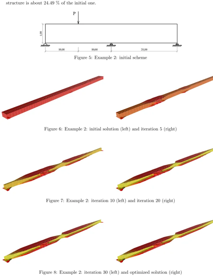
The second example (figure 5) is a beam 40 m long and 1 m high. It is supported on the left edge, on the center and on the right edge. The horizontal deformation is not restricted. Furthermore, a vertical punctual load of 104 _kN _{is applied in the middle of the left span. The steel has the same properties as} in example 1 but now the mesh is made up of 60×12 = 720 elements. The total weight of the optimized structure is about 24.49 % of the initial one.

Figure 5: Example 2: initial scheme

Figure 6: Example 2: initial solution (left) and iteration 5 (right)

Figure 7: Example 2: iteration 10 (left) and iteration 20 (right)

(9)

8. Conclusions

We present a minimum weight formulation for structural topological optimization with local stress con-straints.

The formulation is based on an optimization method wich includes a conventional FEM approach with simple modifications.

The presented optimization approach does not require neither artificial parameters nor stabilization techniques. Intermediate densities are not penalized neither.

The objective function and the constraints have a clear physical interpretation from an engineering point of view. In addition, another kind of constraints could be used (displacementes, vibration frequencies) and several load cases could be analysed simultaneously.

From a mathematical point of view the formulation is very robust. However, this approach implies a high number of non linear constraints wich implies a large amount of data storage.

9. Acknowledgements

This job has been partially supported by Grant Numbers DPI2002–00297 and DPI2004–05156 of the”Ministerio de Ciencia y Tecnolog´ıa” of the Spanish Government, by Grant Numbers PGIDIT03– PXIC118001PN and PGIDIT03–PXIC118002PN of the ”Dirección Xeral de I+D”of the ”Conseller´ıa de Innovación, Industria e Comercio” of the ”Xunta de Galicia”, and by research fellowships of the ”Universidade da Coruña”and the”Fundación de la Ingenier´ıa Civil de Galicia”.

10. References

[1] Bendsøe M.P., Optimization of structural topology, shape, and material. Springer–Verlag, Heidel-berg, 1995.

[2] Muiños I., Optimización Topológica de Estructuras: Una Formulación de Elementos Finitos para la Minimización del Peso con Restricciones en Tensión. Technical Report, ETSICCP, Universidade da Coruña, A Coruña, 2001.

[3] Navarrina F., Una metodolog´ıa general para optimización estructural en diseño asistido por orde-nador,PhD Thesis, Universidad Politécnica de Cataluña, Barcelona, 1987.

[4] Ministerio de Fomento, NBE EA–95 Estructuras de acero en edificaci´on. Centro de Publicaciones del Ministerio de Fomento, Madrid, 1998.

[5] Duysinx P., Topology optimization with different stress limits in tension and compression. Inter-national report: Robotics and Automation, Institute of Mechanics, University of Liege, Belgium, 1998.

[6] Hernández S., Métodos de Diseño Óptimo de Estructuras,Colegio de Ingenieros de Caminos, Canales y Puertos, Madrid, 1990.

[7] Navarrina F. and Casteleiro M., A general methodologycal analysis for optimum design. Interna-tional Journal of Numerical Methods in Engineering, 1991, 31, 85–111.

[8] Sigmund O., Design of material structures using topology optimization, Ph. D. Thesis, DCAMM Report S.69, Department of Solid Mechanics, DTU, Lyngby, 1994.

[9] Oñate E., Cálculo de Estructuras por el Método de Elementos Finitos: Análisis estático y lineal, CIMNE, second edition, Barcelona, 1995.

[10] Yang R. J., Stress-based topology optimization,Structural Optimization, 1996, 12, 98–105. [11] Cheng G.D. and Guo X.,ε-relaxed approach in structural topology optimization,Structural

(10)

[12] Bendsøe M.P. and Kikuchi N., Generating optimal topologies in structural design using a homog-enization method, Computer Methods in Applied Mechanics and Engineering, 1988, 71, 197–224.

[13] Ramm E., Maute K. and Schwarz S., Adaptive topology and shape optimization, Computational Mechanics: New trends and applications, Proc. of the IV-World Conference on Computational Mechanics (CD-ROM), S. Idelshon, E. O˜nate & E. Dvorkin (Eds.), CIMNE, Barcelona, 1998.

[14] Navarrina F., L´opez S., Colominas I., Bendito E. and Casteleiro M., High order shape design sensitivity: A unified approach, Computer Methods in Applied Mechanics and Engineering, 2000, 188, 681–696.

[15] Navarrina F., Tarrech R., Colominas I., Mosqueira G., Gómez-Calviño J. and Casteleiro M., An efficient MP algorithm for structural shape optimization problems, Computer Aided Optimum Design of Structures VII, S. Hernández & C.A. Brebbia (Eds.), WIT Press, 2001, Southampton, 247–256.

[16] Muiños I., Colominas I., Navarrina F. and Casteleiro M., Una formulación de m´ınimo peso con restricciones en tensión para la optimización topológica de estructuras, Métodos Numéricos en Ingenier´ıa y Ciencias Aplicadas, E. Oñate, F. Zárate, G. Ayala, S. Botello & M.A. Moreles (Eds.), CIMNE, 2002, Barcelona, 399–408.