Stock return comovements and integration within the Latin American integrated market

SERIE DO C UM ENTO S DE TRA BA JO

No . 1 5 4

A b ril d e 2 0 1 4

STOCK RETURN COMOVEMENTS AND INTEGRATION WITHIN

THE

LATIN AMERICAN INTEGRATED MARKET

Stock return comovements and integration within

the Latin American integrated market

Carlos Castro

Nini Johana Mar´ın

a. Faculty of Economics, Universidad del Rosario, Colombia.

b. Faculty of Engineering, Universidad de Medell´ın, Colombia.

March 25, 2014

Abstract

Financial integration has been pursued aggressively across the globe in the last fifty years; however, there is no conclusive evidence on the diversification gains (or losses) of such efforts. These gains (or losses) are related to the degree of comovements and synchronization among increas-ingly integrated global markets. We quantify the degree of comovements within the integrated Latin American market (MILA). We use dynamic correlation models to quantify comovements across securities as well as a direct integration measure. Our results show an increase in comovements when we look at the country indexes, however, the increase in the trend of correlation is previous to the institutional efforts to establish an inte-grated market in the region. On the other hand, when we look at sector indexes and an integration measure, we find a decreased in comovements among a representative sample of securities form the integrated market.

Keywords: comovements, correlation, market integration. JEL Classification: G11,G12,G15.

1

Introduction

Within the last fifty years there has been a profound and decisive interest in facilitating financial mobility across the globe. The interest has been nurtured by the quest for higher premiums taking advantage of the good performance of different markets at different points in time. On the other hand, there is an explicit interest in integrating negotiation platforms across the main financial centers in developed countries (OMX 1997, Euronext 2001, Euronext-NYSE 2006). Even emerging markets have not staid far behind these integration ef-forts (MILA 2011, SADC). The integration of financial markets both implicit

or explicit represents important investments and challenges (technological and regulatory) but provides opportunities and benefits.1 _{It is common to find the}

following justifications in explicit efforts to integrate financial markets at the regional or global scale: reduction of transaction cost due to shared platforms, increased liquidity and depth, a better risk-return balance, increase access to financial products, among others. A broader range of different assets, within mean-variance portfolio technology, can lead to the ex-ante belief of an increase of diversification benefits, as it is commonly advertised in explicit efforts to in-tegrate markets. However, comovements and synchronization of markets can limit any potential diversification benefits. Financial economist consider that markets are internationally integrated if the reward for risk is identical regard-less of the market one trades in. Under this scenario market integration explicit or implicit can have a negative effect on diversification.

Comovements are indicative of the effect of market integration and in some extent of the viability of active portfolio management in an international con-text Kavussanos et al. (2002); Isakov and Barras (2003); Driessen and Laeven (2007); Cowan and Joutz (2006); Bekaert et al. (2009). Within a more brother literature that encompasses both portfolio choice literature as well as risk mea-surement some articles examine the merits of international diversification Ang and Bekaert (2002); Das and Uppal (2004); Guidolin and Timmermann (2008), Kaplanis and Schaefer (1991); You and Daigler (2010); Chiou (2008); Berger et al. (2011)). The results are mixed results, there is evidence that emerging or frontier markets provide important gains of holding a global portfolio. How-ever, they also find consistently that correlation across equity markets reduces the gains from diversification for the US investor. Furthermore, when solving the dynamic portfolio problem they find that any gain is strongly state dependent. More recently, Gallali and Kilani (2010) and in particular Christoffersen et al. (2010), use recent models (scalar BEKK, DCC, DECO and a dynamic t-copula) to quantify conditional correlations, and find evidence of high correlation within and across developed and emerging markets. This last paper argues that de-pendence in the tails of the return distributions has increased at a greater pace in developed markets but it is still relatively low in emerging markets, therefore they argue that diversification benefits has fallen across developed markets and remain intact for emerging markets.

Another approach if to measure the extend of financial integration. As men-tioned previously fully integrated international markets (or syncronization ac-cross markets) is expected to have negative effects on the possibility of exploit-ing diversification strategies.Bruneau and Caicedo-llano (2009) analyze different measures of market comovements using principal component analysis and de-velop a measure of integration based on the correlation of returns across markets to the average percentage of variance explained by the first principal compo-nent. The authors find that both developed and emerging markets experienced and increased in comovement during the period of study and provide a measure

1

of diversification in both cases.

The aim of this paper is to examine comovements across a representative group of securities from the integrated Latin American market (MILA). As mentioned previously, market integration provides a broader access to equities, but at the same time comovements across these markets can limit any benefit from diversification. Since we will be looking at the evolution of the markets in-volved in the Latin American integrated market (Chile, Colombia and Peru) we will use recent statistical methods to estimate dynamic correlation between the securities across countries and sectors, as well as a direct integration measure.

Results indicate that over the period 2008-2013, there is an increase in cor-relation in the three markets when we look a the country indexes. However, this increase is more pronounced for Chile and Colombia than Peru. In the same period we find a different result when we build indexes base on economic sectors, this is important because one of the motivations behind the MILA was to take advantage of the heterogeneity among the sectors present in the stock market of the three countries. For sectors we find either a constant correlation or a de-crease in correlation over the sample. This last result cast a shadow of doubt on the extend of integration. Furthermore, when we find a downward trend on the integration measure, we arrive at a similar conclusion. The result is encouraging for investor and for the MILA market because it indicates a broader range of available asset with strong possibilities of diversification opportunities and that full integration is still far away or at least it is to early to determine.

The outline of the paper is as follows: Section 2 presents a short overview of the integrated Latin American market. Section 3 presents the different method-ologies used to: filter out correlation between the sample of securities and mea-sure integration between the markets. Section 4 provides a summary of the most important results. Section 5 concludes.

2

Latin American Integrated Market

All MILA negotiations are done in local currency without having to leave their home countries and orders are transmitted through local intermediary. Al-though MILA became operational on 30 May 2011, its origins date back to 2007 when the Colombia Stock Exchange (BVC) and the Lima Stock Exchange (BVL) proposed a model of integration. Then these exchange markets invited the Chilean stock exchange (BCS) to participate in the integration process.

Currently, MILA is the first market by number of listed companies in Latin America, the second largest in terms of market capitalization and third in trad-ing volume. Figure 1 reports the distribution, by country and industry, of a sample of 37 securities that make up the S&P MILA 40 index, during the first trimester of 20132_{. During this period the country with most participation, in}

the S&P MILA 40 index, is Chile (50%), and then Colombia (32%) and finally is Peru (18%). One of the distinguishing features of the integrated market is that

2

there is important sectoral differences across countries, for example Banking and Finance is an important sector for both Colombia and Chile, unlike Peru where Mining has a higher importance. Furthermore there are sector that are specific to some countries, like technology and industrial in Chile and food in Colombia.

Ex-ante financial market integration is thought to have substantial trans-action cost benefits for many of the parties involved (investors, financial insti-tutions, markets, issuers). In particular, the benefits mentioned in the official information of the MILA market for investors (our main concern) are: a) easier and cheaper access for retail investors, b) larger base of financial instruments at their disposal, c) greater depth and liquidity, d) increase in the possibility to diversify portfolios, e) a better balance between risk and return and d) unique access point to the regional market for foreign investors. Many of these benefits are to some degree measurable directly from the market data (subject to data availability), for example using the cost of trade, stock prices, volumes, bid and ask spreads. Based on the experience on Euronext, Pagano and Padilla (2005) note that there are two types of transaction costs that may be affected from the merger of different transaction platforms: Explicit cost, such as commissions, compensation and liquidation cost, and technological cost. If available the evo-lution of such cost can give a precise measure of the benefits of the merger. Implicit cost, such as a reduction in the bid-ask spread through higher liquidity or gains from diversifications. Gains on the latter are not directly available, nonetheless our strategy is to measure the degree of comovements between the securities of the integrated market.

3

Measuring comovements and market

integra-tion

Understanding and quantifying comovements across assets is an essential issue in portfolio optimization, in particular, it is vital to understand the possibility of exploiting diversification benefits. On the other hand, measuring comove-ments also plays a role in determining the extend of integration across financial markets. We will use two methodologies, first we determine if there has been an increase in co-movements across the markets that make up the Latin American integrated market (MILA) and its relationship to the integration efforts within these three markets. Second, we use a market integration measure based on co-movements of the individual stocks to investigate to what extend are the explicit integration efforts reflected in the market data.

3.1

Dynamic conditional correlation

Engle, Bollerslev and co-authors have introduced different methods to estimate conditional correlations.

Most of the methods proposed and surveyed in the next paragraphs seek to parametrize the covariance matrix of a set of random variables, conditional on a set of observable state variables, that typically include past realization of the variables of interest (in our case returns).

Letri,tdenote the return of assetiat timet, follow the process (i= 1, . . . , n,

t= 1, . . . , T).

ri,t=µi,t+εi,t=µi,t+σi,tzi,t (1)

wherezi,tis a standard normal random variable,σ2i,tandµi,tare the conditional

variance and mean, respectably.

Covariances between assetsiandj, follows a first order scalar MGARCH (Engle and Kroner (1995),Engle (2002), Tse and Tsui (2002)),

σ2i,j,t=λi,j+αεi,t−1εj,t−1+βσ

2

i,j,t₋1. (2)

whereεi,tis the return innovation. The multivariate representation of the model

is as follows

Σt= Λ +αεt−1εt−1+βΣt−1 (3)

There are a total of n(n₂+1)+ 2 parameters to estimates, most of the parameters are in the intercept (λi,j’s).

Even though the scalar MGARCH can accommodate many assets, Cappiello et al. (2006) shows that restrictions on the dynamics of the variance covariance process do not capture the persistence effects of correlation; for this reason we rather concentrate on the Dynamic Conditional Correlation Model (DCC), Engle (2002), and in particular the mean reverting version of this model. The covariance matrix can be written as a function of the correlation matrix and a diagonal matrix of the variances (spectral decomposition), Σt=DtΓtDt with

D2t =diag(Σt). LetQt denote an approximation to the correlation matrix Γt

hence we can denoteQtas a quasi-correlation. The quasi-correlation process is

dynamically described by,

Qt= Ω +αζt−1ζ

′

t₋1+βQt−1 (4)

whereζtis the vector of standardized residualsεi,t/

√

σ2

i,i,t. There are the same

number of parameters to estimate as in the previous model n(n₂+1)+ 2, how-ever we can use the uncondicional representation of the model and the sample covariance of the standardized residuals to reduce the number of parameters.

ˆ

Ω = (1−α−β) ¯R,R¯= _T1

T

∑

t=1 ζt−1ζ

′

t₋1 (5)

the previous strategy gives us a more parsimonious model to estimate as well as the mean reverting version of the DCC model.

Qt= ¯R+α(ζt−1ζ

′

The principle behind the mean reverting DCC is that when returns are mov-ing in the same direction, either both movmov-ing up or down, the correlation will rise above its average level and remain there for a while. Gradually this phe-nomenon, on the the returns, will decay and correlations will fall back to their long run average. The parametersαandβ determine the speed of the adjust-ment.

The elements ˆqi,j,t of the matrix Qt are the quasi-correlation that we can

transform into exact correlations, by ˆρi,j,t= ˆ qi,j,t

√_qˆ

i,i,tqˆj,j,t

. The stochastic process described by the pairwise exact correlationsρi,j,tis our main object of interest.

Although DCC has been used extensively for the analysis of dynamic con-ditional covariances and correlations across investments instruments, a recent article Caporin and McAleer (2013) points out some of the limits of the DCC rep-resentation for estimation and forecasting time-varying conditional correlations. Among the issues pointed out in the paper is the lack of a proper discussion on the stationarity conditions or the asymptotic properties of the estimators in most representations or extensions of DCC. As stress by the author this crit-icism does entire rule out the possibility of using DCC as a filter of dynamic conditional correlations; therefore, the recent criticism does not invalidate our effort of using DCC to obtain time-varying measures of the dependence across the stocks that are part of the integrated Latinamerican market (MILA).

In order to disentangle a possible trend between the time-varying correlations within the MILA we use a smooth transition model. This methodology was introduced by Granger and Terasvirta (1993) and has been applied to study equity market co-movements by Chelley-Steeley (2008) and A. and K. (2011). It allows us to estimate when one the structural changes first occurred and its duration, based solely on time-varying correlations obtained with the DCC model. Following to A. and K. (2011), we first calculates equity market weekly return correlations by country and sector. The smooth transition model is applied to bivariate equity market dynamic conditional correlations which have been derived using the DCC-GARCH model. We consider the a logistic smooth transition regression model for the conditional correlation time series ˆρi,j,t,

ˆ

ρi,j,t=θ+κSt(γ, τ) +µt (7)

whereµtis a zero mean stationaryI(0) process. The smooth transition between

the two correlation regimes is controlled by the logistic functionSt(γ, τ) defined

as:

St(γ, τ) =

(

1 +exp(

−γ(−¨τ)))−1 (8)

abrupt for large values ofγ. The model assumes that conditional correlations change from one stationary regime to another stationary regime with mean a

α+β. Ifβ >0 the conditional correlations move upward, whereas ifβ <0 the conditional correlations move downward. Before applying the smooth transition model, we test if the conditional correlations are stationary. If they are, then no change in intercept occurs and the above smooth transition model is not applicable.

3.2

Indicator of financial integration

There are different approaches to measure financial integration based on equity data. We use a measure of integration based on Bruneau and Caicedo-Llano (2006). The measure is based on market co-movements. The first step is to mea-sure the main factors explaining the cross-sectional equity returns with principal components analysis (PCA), and construct a measure of integration based on the average percentage of variance explained by the first factor ˆF1 extracted

from the PCA. The unit of analysis are the equity returns ri,t that obey the

following multiple factor structure:

ri,t=ai+ K

∑

j=1

bi,jfj,t+εi,t (9)

where ai is the expected return on asset i, fj,t is the realization at time t of

the common factorj,bi,jthe sensitivity of assetito the movements of factorj,

εi,t is a noise term representing the idiosyncratic risk and K is the number of

common factors representing the systematic and local systematic components of risk. Factors can be estimated with factor analysis (FA) or principal component analysis. When there are a large number of data and N → ∞, FA and PCA are equivalent. However, we are in a setting with only few variables, therefore PCA and FA provide similar results, but are not equivalent. The integration measure (It), proposed by Bruneau and Caicedo-Llano (2006), is defined as:

It=

1

N

N

∑

i=1

ˆ

ρ2(ri,t₋H,t,Fˆ1,t₋H,t) (10)

where ˆF1,t−H,tis the first component estimated with a PCA on the correlation

of returns for a set ofN assets,ri,t−H,t is the vector of returns of asseti from

time t−H to time t and ρ2 is the squared correlation of two variables. The periods when the returns are highly correlated to the first component can be interpreted like periods of high integration.

3.3

The data

represented in the index S&P MILA 40. Missing values for periods not operat-ing in a given market due to holidays were replaced by the precedoperat-ing data in order to guarantee five-day weeks. The source of data is Bloomberg. For the dynamic correlation analysis we build US dollar value, country and industry indexes (see section 6). However when we use the integration measure we use the individual securities measured in US dollar returns. In general, the results are not sensitive to the currency denomination both at the individual securities level or for the indexes. We build sector indexes because they represent, as men-tioned previously, a relevant risk group for the integrated market, furthermore one of the reasons for the regional markets to integrate was on the perceived notion that the integrated market would increase the variety of assets available to local investors.

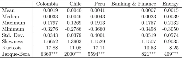
Tables 1 and 2 provide descriptive statistics on the country and sector in-dexes. The weekly returns for the group of indexes is negatively skewed and strongly asymmetric, therefore this is consistent with leptokurtic and heavy tailed distributions. In all cases we reject the null hypothesis (of the Jarque-Bera test) that the distribution is gaussian.

4

Empirical Results

As an initial step in estimating dynamic conditional correlations we must de-garch each return series. A GARCH(1,1) model with Gaussian errors, was employed for each security or index, to control for second moment time de-pendence3_{. The degarching is necessary to obtain unbiased estimates of the}

dynamic correlations, based on the estimated standardized residuals ˆζi,t we fit

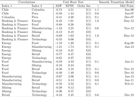
the mean reverting DCC model. Table 3 shows the estimated parameters of the DCC model, the magnitude ofβ indicates a strong mean reversion in most of the cases. Table 4 contains the stationarity test on the conditional correlations across the pair of countries or sectors. The fifth column of the table indicates where the series is taken as stationaryI(0) or non-stationaryI(1).

As mentioned before in order to identify a trend in correlation and further-more see if this trend is consistent with the explicit efforts toward the integration of these Latin American markets we estimate a smooth transition model on the correlation estimates obtained from the DCC model,ˆρi,j,t. However, as argued

by A. and K. (2011) fitting the smooth transition model is informative only if there is a significant change in the trend, therefore if the conditional correla-tions are stationary there is no point on fitting the model. We estimate and report (table 4) the estimates of the smooth transition model for the time series of conditional correlation that are non-stationary. The estimated parameterγ

indicates the smoothness of the transition, lower values indicate a soft transition from state one to state two. The last column in table 4, indicates the month that is determined as the mid point of the transition. As mentioned in the

in-3

troduction, although the integration process started in 2007, the MILA market only started operations on May 30, 2011. As to the date of the transitions we find mixed results:

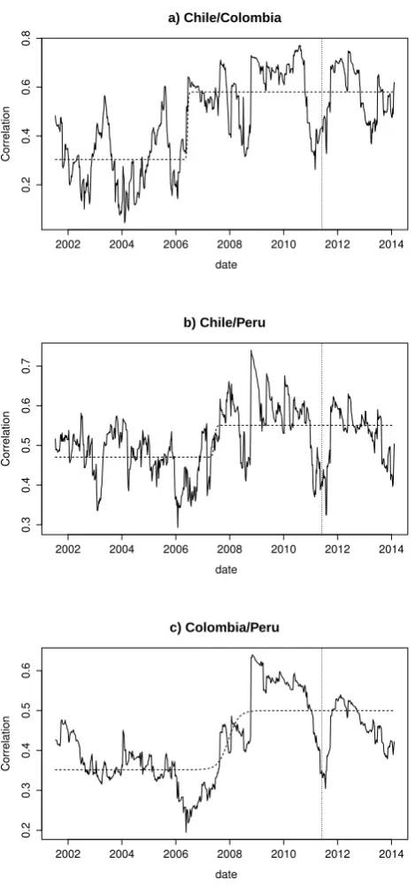
For countries the change in the trend in correlations is stronger for Colombia and Chile (that is an increase in correlation) and much weaker (but still posi-tive) between Colombia and Peru, and Chile and Peru. However, these changes occurred over the course of 2006 and 2007. The change was more abruptly for Colombia and Chile and smoother and subtle in magnitude for the other coun-try pairs (figure 2).

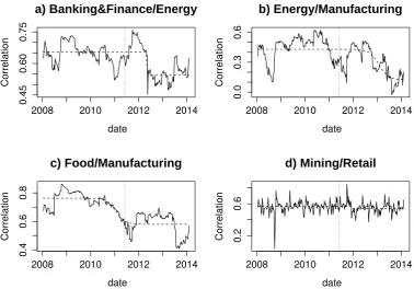
For sectors; first, as indicated in table 4 there are nine sector pairs where we find no evidence of a change in the trend in correlation over the sample period. Second, the change in the trend is negative and it is in general in the latter part of the sample, therefore is could possibly be related to the formal integration process. Figure 3 presents the time series of correlations for a sample of sectors that are representative of the overall trend. The first three plots (a,b,c) repre-sent those pairs of sectors where we find a significant change in the trend. The change in the trend is captured by the dashed line. For example, energy and banking & finance in the first part of the sample have a correlation of around 0.67, but afterwards there is an abrupt transition around May-2012, after which correlation is around 0.55. Food and manufacturing in the first part of the sample have a correlation of around 0.78, but afterwards there is an smooth transition, starting in the middle of 2010 and a mid point around Jan-2011, after which correlation is around 0.58. The last plot c, represents those pairs of sectors where the time series of correlations are stationary, where the smooth transition model is meaningless and correlation is more or less constant, for mining and retail at around 0.57 throughout the sample.

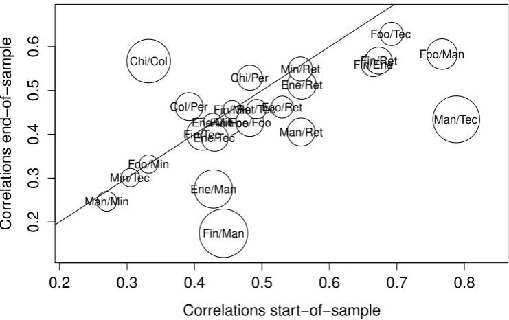
In general, we find that correlation has been increasing at the country level and it has remained the same or decreased at the sector level. We also find no compelling evidence that the change in the trend in correlations is strongly related to the integration of the capital markets of Colombia, Chile and Peru. Figure 4 presents the results for all pairwise correlations in a concise manner: the data indicates the average correlations observed at the beginning (2008-2009) and the end (2012-2014) of the sample, where the size of the bubbles reflects the standard deviation of correlations over the full sample. Correlations above (below) the 45◦ _{line indicate strong evidence that correlations have}

in-creased (dein-creased) over the sample; correlations that are on the 45◦_{indicate no}

significant change4. Not surprisingly we find that the country correlations are above the 45◦ _{line and the sector correlations are below. This is not a strange}

phenomenon to expect in these developing capital markets where the risk per-ception of global investors can lead to strong comovements on similar regional emerging markets, such is the case of Colombia, Chile and Peru. However, as we saw in figure 1 at a sector level, the integrated market provides an increased sector-wide variation to each of the local markets.

4

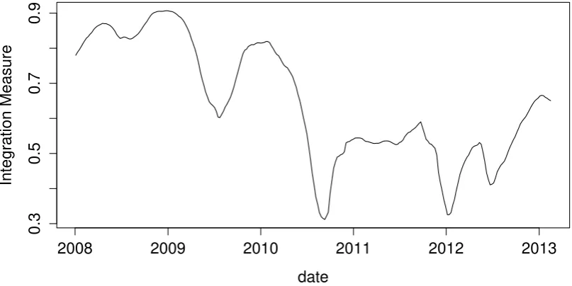
We provide complementary evidence on the scope of integration between the three markets using the proxy of integration proposed by Bruneau and Caicedo-Llano (2006). Figure 5 plots the evolution of the integration measure

It (expression 10). Recall that this measure is based on the individual stocks

for the sample of securities that we have collected for the three countries. The measure indicates a stronger integration at the beginning of the sample than at the end of the sample, this result is contradictory to the explicit institutional effort toward integration of the three markets, however the result is consistent to what we observed with respect to the sector indexes in figures 3 and 4.

5

Conclusions

For investors co-movements between assets and in particular correlation carry information of the possible diversification benefits of investing across borders and in different sectors. We look at the co-movements of stocks, at the index level but also at the individual securities, for Chile, Colombia and Peru. These countries are specially interesting because of the explicit efforts of integrating their stock markets. Effort that have led to the creation of the Latin American Integrated Market (MILA).

Our results indicate that over the period 2008-2013, there is an increase in correlation in the three markets when we look a the country indexes. However, this increase is more pronounced for Chile and Colombia than Peru. In the same period we find a different result when we build indexes base on economic sectors, this is important because one of the motivations behind the MILA was to take advantage of the heterogeneity among the sectors present in the stock market of the three countries. For sectors we find either a constant correlation or a decrease in correlation over the sample. This last result cast a shadow of doubt on the extend of integration. Furthermore, when we find a downward trend on the integration measure, we arrive at a similar conclusion. The result is encouraging for investor and for the MILA market because it indicates a broader range of available asset with strong possibilities of diversification opportunities and that full integration is still far away or at least it is to early to determine.

References

A., L. and K., S. (2011). U.s. and latin american stock market

link-ages.

Journal of International Money and Finance

, 30:13411357.

Ang, A. and Bekaert, G. (2002). International asset allocation with

regime shifts.

Review of Financial Studies

, 15(4):1137–1187.

Bekaert, G., Hodrick, R., and Zhang, X. (2009). International stock

comovements.

Journal of Finance

, 64(6):2591–2626.

Berger, D., Pukthuanthong, K., and Yang, J. (2011). International

diversification with frontier markets.

Journal of Financial

Eco-nomics

, 101:227–242.

Bruneau, C. and Caicedo-Llano, J. (2006). Comovements of

interna-tional equity markets and financial integration measures.

Working

Paper

, 1:1–45.

Bruneau, C. and Caicedo-llano, J. (2009). Co-movements of

in-ternational equity markets: a large-scale factor model approach.

Economics Bulletin

, 29:1484–1500.

Caporin, M. and McAleer, M. (2013). Ten things you should know

about dcc. Working Paper.

Cappiello, L., Engle, R., and Sheppard, K. (2006). Asymmetric

dynamics in the correlations of global equity and bond returns.

Journal of Financial Econometrics

, 4:537–572.

Chelley-Steeley, P. (2008). Modelling equity market integration

us-ing smooth transition analysis: a study of eastern european stock

markets.

Journal of International Money and Finance

, 24:818831.

Chiou, W. (2008). Who benefits more from international

diversifi-cation?

Journal of International Financial Markets, Institutions,

and Money

, 18:466482.

Christoffersen, P., Errunza, V., and Jacobs, K., J. X. (2010). Is the

potential for international diversification disappearing?

Discus-sion Paper, University of Toronto

, 1:1–41.

Cowan, A. and Joutz, F. (2006). An unobserved component model

of asset pricing across financial markets.

International Review of

Das, S. and Uppal, R. (2004). Systemic risk and international

port-folio choice.

Journal of Finance

, 59(6):2809–2834.

Driessen, J. and Laeven, L. (2007). International portfolio

diversifi-cation benefits: Cross-country evidence from a local perspective.

Journal of Banking & Finance

, 31(6):1693–1712.

Engle, R. (2002). Dynamic conditional correlation: A simple class

of multivariate garch models.

Journal of Business and Economic

Statistics

, 20:339–350.

Engle, R. and Kroner, K. (1995). Multivariate simultaneous

gener-alized arch.

Econometric Theory

, 11:122–150.

Gallali, M. and Kilani, B. (2010). Stock markets volatility and

in-ternational diversification.

Journal of Business Studies Quarterly

,

1(4):21–34.

Granger, C. and Terasvirta, T. (1993).

Modelling Nonlinear

Eco-nomic RelationshipsGranger1993

. Oxford University Press.

Guidolin, M. and Timmermann, A. (2008). International asset

al-location under regime switching, skew and kurtosis preferences.

Review of Financial Studies

, 21(2):889–935.

Isakov, D. and Barras, L. (2003). How to diversify internationally?

a comparison of conditional and unconditional asset allocation

methods.

Financial Markets and Portfolio Management

, 17:194–

212.

Kaplanis, E. and Schaefer, S. (1991). Exchange risk and

interna-tional diversification in bond and equity portfolios.

Journal of

Economics and Business

, 43:287–307.

Kavussanos, M., Marcoulis, S., and Arkoulis, A. (2002).

Macroeco-nomic factors and international industry returns.

Applied

Finan-cial Economics

, 12:923–931.

MSCI (2013). Msci index calculation methodology. Technical report,

MSCI Inc.

Tse, Y. and Tsui, A. (2002). A multivariate garch model with

time-varying correlations.

Journal of Business and Economic Statistics

,

20:351–362.

You, L. and Daigler, R. T. (2010). Is international diversification

really beneficial?

Journal of Banking & Finance

, 34:163173.

6

Appendix

We follow the MSCI price index methodology MSCI (2013) to construct coun-try, sector and country/sector indexes based on the sample of stocks that are included in the index of the Latin American Integrated market (MILA).

The index in a particular currency (US dollars) is obtained by applying the change in the market performance to the previous period index level.

Indext= Indext₋1

Market Cap USDt

Market Cap USDt₋1

(11)

where the market capitalization contains the value of all the stocks belong-ing to that particular index. Let SIndex denote the total number of stocks

that belong to a particular index (for example, Chile, Banking and Finance or Colombia/Retail).

Market Cap USDt= SIndex

∑

i=1,t

No. of Sharesi,tPricei,t

FXratet

(12)

where FXratetis the FX rate of the price currency of stockiversus de US dollar

Table 1: Descriptive statistics of the weekly returns on the country and sector indexes

Colombia Chile Peru Banking & Finance Energy Mean 0.0019 0.0040 0.0041 0.0007 0.0015 Median 0.0033 0.0046 0.0043 0.0023 0.0039 Maximum 0.1797 0.1269 0.1913 0.1757 0.2132 Minimum -0.3276 -0.2786 -0.3660 -0.3498 -0.3050 Std. Dev. 0.0343 0.0379 0.4001 0.0519 0.0574 Skewness -1.6652 -1.3903 -1.1529 -1.1507 -0.9035 Kurtosis 17.88 11.08 17.11 10.53 8.25 Jarque-Bera 6369∗∗∗ ₂₀₀₀∗∗∗ ₅₅₉₄∗∗∗ ₈₂₁∗∗∗ ₄₀₉∗∗∗

Notes:∗_,∗∗_{, and}∗∗∗_{indicate a significance at the 10, 5 and 1% level, respectively.}

Table 2: Descriptive statistics of the weekly returns on sector indexes

Food Manufacturing Mining Retail Technology Mean 0.0014 0.0021 -0.0025 0.0009 0.0030 Median 0.0021 0.0016 -0.0012 0.0018 0.0049 Maximum 0.1311 0.0839 0.2473 0.1464 0.1181 Minimum -0.1886 -0.1838 -0.2671 -0.2740 -0.1922 Std. Dev. 0.0368 0.0328 0.0538 0.4009 0.0347 Skewness -0.4949 -1.2049 -0.0529 -1.1394 -0.8418 Kurtosis 6.02 8.71 6.22 11.00 7.36 Jarque-Bera 134∗∗∗ ₅₁₀∗∗∗ ₁₃₈∗∗∗ ₉₁₆∗∗∗ ₂₈₉∗∗∗

Table 3: Estimated parameters of mean reverting DCC-GARCH model, for pairs of countries and sector indexes

Index 1 Index 2 α β

Chile Colombia 0.054 0.874∗∗∗

Chile Peru 0.008 0.975∗∗∗

Colombia Peru 0.019 0.870∗∗∗

Banking & Finance Energy 0.021 0.954∗∗∗

Banking & Finance Food 0.078∗∗∗ _0.648∗∗∗

Banking & Finance Manufacturing 0.019 0.973∗∗∗

Banking & Finance Mining 0.032 0.868∗∗∗

Banking & Finance Retail 0.010 0.984∗∗∗

Banking & Finance Technology 0.017 0.714 Energy Food 0.010 0.979∗∗∗

Energy Manufacturing 0.024 0.882∗∗∗

Energy Mining 0.016∗∗∗ _0.833

Energy Retail 0.158∗∗∗ _0.447

Energy Technology 0.095∗∗∗ _0.555∗∗∗

Food Manufacturing 0.023 0.919∗∗∗

Food Mining 0.023∗∗∗ _0.827∗

Food Retail 0.009 0.802 Food Technology 0.025 0.697∗∗∗

Manufacturing Mining 0.020∗∗∗ _0.804

Manufacturing Retail 0.697∗∗∗ _0.612∗∗∗

Manufacturing Technology 0.025 0.953∗∗∗

Mining Retail 0.092∗∗∗ _0.381

Mining Technology 0.042∗∗∗ _0.549∗∗∗

Retail Technology 0.128∗∗∗ _0.362∗∗∗

Table 4: Smooth transition model for pairwise correlations

Correlations Unit Root Test Smooth Transition Model Index 1 Index 2 ADF KPSS Order Int. γ Mid Point Chile Colombia -0.74 4.51 I(1) 1.1 Jun-06

Chile Peru -0.58 1.44 I(1) 0.6 Jun-07

Colombia Peru -0.41 3.28 I(1) 0.1 Dec-07 Banking & Finance Energy -0.45 1.91 I(1) 1.6 May-12 Banking & Finance Food -0.68 0.26 I(0)

Banking & Finance Manufacturing -1.42 2.25 I(1) 0.6 Nov-12 Banking & Finance Mining -0.12 0.18 I(0)

Banking & Finance Retail -0.69 1.63 I(1) 1.6 May-12 Banking & Finance Technology -0.55 0.06 I(0)

Energy Food -1.10 1.20 I(1) 0.1 Aug-08 Energy Manufacturing -1.21 1.74 I(1) 0.1 Jan-13 Energy Mining -0.16 0.21 I(0)

Energy Retail -0.77 0.47 I(0) Energy Technology -0.65 0.37 I(0)

Food Manufacturing -0.59 3.43 I(1) 0.1 Jan-11 Food Mining -0.16 0.24 I(0)

Food Retail -0.56 2.18 I(1) 0.1 Nov-12 Food Technology -0.40 1.40 I(1) 9.6 Dec-10 Manufacturing Mining -0.67 2.06 I(1) 0.1 Jan-13 Manufacturing Retail -0.51 3.14 I(1) 0.6 Jan-11 Manufacturing Technology -0.76 3.52 I(1) 0.1 Feb-11 Mining Retail -0.38 0.12 I(0)

Mining Technology -0.36 0.57 I(0)

Retail Technology -0.43 2.45 I(1) 0.6 Dec-10

Notes: The Augmented-Dickey-Fuller (null hypothesis unit root) and KPSS (null hypothesis no unit root) unit root test are performed using a lag structure determined form information criteria, columns three and four provide the statistic for the unit root test. Column five determines whether the correlation time series is stationaryI_{(0) or}

non-stationaryI_{(1). For those asset pairs where the correlation time series is non-stationary, column six and seven}

2002 2004 2006 2008 2010 2012 2014

0.2

0.4

0.6

0.8

a) Chile/Colombia

date

Correlation

2002 2004 2006 2008 2010 2012 2014

0.3

0.4

0.5

0.6

0.7

b) Chile/Peru

date

Correlation

2002 2004 2006 2008 2010 2012 2014

0.2

0.3

0.4

0.5

0.6

c) Colombia/Peru

date

Correlation

2008 2010 2012 2014

0.45

0.60

0.75

a) Banking&Finance/Energy

date

Correlation

2008 2010 2012 2014

0.0

0.3

0.6

b) Energy/Manufacturing

date

Correlation

2008 2010 2012 2014

0.4

0.6

0.8

c) Food/Manufacturing

date

Correlation

2008 2010 2012 2014

0.2

0.6

d) Mining/Retail

date

Correlation

0.2

0.3

0.4

0.5

0.6

0.7

0.8

0.2

0.3

0.4

0.5

0.6

Correlations start−of−sample

Correlations end−of−sample

Chi/Col

Chi/Per

Col/Per

Fin/Ene

Fin/Foo

Fin/Man Fin/Min

Fin/Ret

Fin/Tec

Ene/Foo

Ene/Man Ene/Min

Ene/Ret

Ene/Tec

Foo/Man

Foo/Min

Foo/Ret

Foo/Tec

Man/Min

Man/Ret

Man/Tec Min/Ret

Min/Tec

Ret/Tec

Figure 4: Average correlations at the beginning and the end of the sample. The size of the bubbles is determined by the sample standard deviation. Smaller bubbles on the 45◦ _{line are indicative of constant correlation throughout the}

2008

2009

2010

2011

2012

2013

0.3

0.5

0.7

0.9

date

Integr

ation Measure