Firm entry, productivity differentials and turnovers in import substituting markets: a study of the petrochemical industry in Colombia

ECONOMÍA

SERIE DOCUMENTOS

No. 42, abril de 2004

Firm Entry, Productivity Differentials and

Turnovers in Import Substituting Markets: A study

of the Petrochemical Industry in Colombia

Luis H. Gutiérrez

Carlos Pombo

BORRADORES DE

INVESTIGACIÓN BORRADORES

DE

del Rosario, 2004.

50 p. : il., cuad., tab. –- (Economía. Serie Documentos, 42). Incluye bibliografía.

ISSN: 0124-4396

INDUSTRIA DEL PETRÓLEO - PRODUCTIVIDAD / INDUSTRIA PETROQUÍMICA –/ PRODUCTOS DEL PETRÓLEO – ASPECTOS ECONÓMICOS / INDUSTRIA DEL PETROLEO – ANÁLISIS ECONÓMI-CO / INDUSTRIA DEL PETRÓLEO – ADMINISTRACIÓN DE PERSONAL – ECONÓMI-COLOMBIA / SALARIOS Y PRODUCTIVIDAD LABORAL / ROTACIÓN EN EL TRABAJO – INDUSTRIA DEL PETRÓLEO – CO-LOMBIA / I. Título / II. Pombo, Carlos.

©Centro Editorial Rosarista © Facultad de Economía

© Autores del libro: Luis H. Gutiérrez, Carlos Pombo

Todos los derechos reservados Primera edición: abril de 2004 ISSN: 0124-4396

F

E

, P

D

T

I

S

M

:

A

C

L

H. G

[email protected]

Facultad de Economía Universidad del Rosario Calle 14 # 4 – 69 Bogotá, Colombia

C

P

*

[email protected]

Facultad de Economía Universidad del Rosario Calle 14 # 4 – 69 Bogotá, Colombia

A

This paper analyses plant entry, total factor productivity growth, average productivity level differentials and turnovers across Colombia’s petrochemical industry for the 1974-1998 period. Results show that successful entrants shaped industry productivity and induced plant restructuring among incumbent plants. There is con-sistent plant heterogeneity across plant cohorts as well as across sub-markets within petrochemicals. Entry flows were steady increasing within plastics regardless of trade policy regimes. Survival rates are remarkably high and consistent over time in medium-size plants meaning that entrants adopted competitive post-entry strategies. Total factor productivity growth decomposition shows that the incumbent effect dominates the turn-over effect. Market share reallocation among continuing plants constitutes an important source of productivity growth. Econometric results suggest that barriers to entry associated with plant technology licensing and depen-dence of imported raw materials deter entry while complementary market variables such as industry productiv-ity levels, growth in housing construction, and fringe competition induce firm entry.

Key Words: Entry, Turnover, Total Factor Productivity, Petrochemical Industry

JEL Classification: O12, D24, O47

1 _{Associate professor, Department of Economics, Universidad del Rosario.}

2 _{Associate professor and director of graduate studies, Department of Economics, Universidad del Rosario.}

* Affiliation: Facultad de Economía, Universidad del Rosario, Address: Calle 14 #4-69, Bogotá, Colombia. Tel: +571-344-5750; fax: +571-3445763

R

El documento analiza la entrada, crecimiento de la productividad total de los factores, diferenciales en productividad promedio y rotación en la industria petroquímica colombiana para el período 1974-1998. Los resultados muestran que los entrantes exitosos dieron forma a la productividad de la industria e indujeron a la reestructuración de las plantas existentes. Existe gran heterogeneidad entre cohortes de empresas así como entre submercados al interior de la industria petroquímica. Los flujos de entrada crecieron constantemente en el sector de plásticos, a pesar de los cambios de política comercial. Las tasas de supervivencia son muy altas y consistentes en el tiempo para las plantas de tamaño mediano, lo que nos lleva a pensar que las empresas entrantes adoptaron para el período post-entrada estrategias competitivas. La descomposición del crecimiento de la productividad total de los factores, muestra que el efecto de las empresas establecidas domina sobre el efecto de rotación de empresas. La redistribución de participación de mercado entre las plantas establecidas hacia las de más alta productividad se constituye en una importante fuente del crecimiento de la eficiencia productiva. Los resultados econométricos sugieren que las barreras a la entrada, asociadas con el licenciamien-to de la tecnología y la dependencia de materias primas importadas disuade la entrada, mientras que variables complementarias del mercado como los niveles de productividad, crecimiento en la construcción de vivienda y competencia periférica inducen la entrada de firmas.

Palabras clave: Entrada, Rotación, Productividad total de los Factores, Industria Petroquímica.

I. I

The petrochemical industry worldwide is formed by vertically-integrated firms. They manu-facture intermediate materials derived from the oil refinement and liquid gas industries that are essential in the manufacture of end products in several industries such as textiles, apparel, domestic appliances, transportation equipment, and housing construction among many others. This industry is intensive in physical capital and along with pharmaceuticals it is also intensive in research and development. Plastics are the most dynamic sub-groups representing around 60% of the industrial uses within petrochemicals because they are close cheap substitutes of other materials currently used in the manufacture of a variety of final goods. On the other hand, production of basic chemicals in Latin America is dominated by multinational enter-prises that entered developing markets during the import substituting industrialization years from the 50s to the 70s in Latin America.

Two types of promoting strategies were implemented in the region. One was the Brazilian-type strategy, which relied on attracting massive direct foreign investment and multinationals through granting non-market entry barriers via tariff protection. Once those firms settled in the market they were expected to pass technological transfers to downstream local industries. The other was the Andean-type (Colombia-Venezuela) strategy, much less aggressive, perhaps be-cause of their domestic market size, that relied both on developing a local basic-chemical industry dependent of crude oil and oil refinement, along with the promotion of foreign direct investment. Several economic policy instruments were used in Colombia three decades ago to promote import-substituting industries such as import licenses, tariffs, tax exceptions applied to specific industries, long-term credits with implicit subsidies, and the direct involvement of government credit institutions in the setup of industrial projects.

Empirical studies on firm entry and turnovers have been focused on the evidence of the OECD cases. The study of Dunne, Roberts, & Samuelson (1988) for the US manufacturing industry is still the most comprehensive country study ever made. Afterwards, there have been just a few efforts in studying firm-level entry, heterogeneity and productivity for the case of developing economies. The collective work of Roberts & Tybout (1996) is the first comprehensive attempt to gather several cases. They include the cases of Morocco, Chile, Colombia, and Mexico. The study of Colombia only covers the 1978-1988 period. Its results clearly are out of date because it leaves the decade of the nineties where the main commercial reforms took place in Colombia since 1959.

The studies of Levinsohn & Petrin (1999) and Pavnick (2002) use the same dataset of Chile from 1980 to 1986. They evaluate manufacturing productivity using the parametric approach of Olley & Pakes (1996). Both papers are more concerned about the econometric advantages of modeling firm level productivity dynamics through stochastic processes than about provid-ing a story regardprovid-ing the effect of entry on local market characteristics and industry develop-ment.3 _{Aw, Cheng, & Roberts (2001) analyzes productivity differentials and plant turnovers for}

3 _{There is an ongoing collective study for Latin America on labor turnover productivity leading by Haltiwanger at the}

the Taiwanese industry based on three census years. Firm-level productivity is estimated through index number methods.

One general drawback of these studies on firm turnover and productivity excepting Olley & Pakes (1996), is that they report generic analyses presenting aggregate measures at two-digits ISIC code where there is no specific explanation regarding the forces behind plant turnover within industries and, more importantly, on what explains turnover differences across industries.

The objective of this paper is three-fold. First, the paper seeks to present an industry case within a semi-industrialized economy in Latin America such as Colombia. The importance of analyzing the petrochemical industry lays down in three reasons: i) as in any developed or developing country it is an industry where barriers to entry may have played a significant role on entry, in particular, scale economies, high fixed costs, and the spending in patented technolo-gies; ii) the development of the petrochemical industry was conditioned by the initial pathway of inward-looking economic development Colombia pursued since the 1950s until the late 1980s. However, the recent export-orientation the industry followed under the economic open-ness program boosted plant entry; iii) petrochemical industries are intertwined in what we call the petrochemical chain [Diagram 1] that introduces an element of plant heterogeneity and productivity differences. Moreover, the technological complexity is increased by the different paths of maturity present in the links along with the petrochemical tree.

Second, the paper seeks to contribute in providing new evidence to shed light on the long-term forces behind entry patterns and plant productivity heterogeneity within an industry with the features above-mentioned. It will so present very detailed plant-level productivity estima-tions that follow state of the art methodologies. Third, the paper looks to test under a variety of econometric specifications what has determined entry in this industry in the long run.

This study makes an effort in analyzing jointly the patterns of entry, the productivity dynamics, and the explanations of what may determine entry in an industry with such special features. To our best knowledge there is no industry study for a developing economy that has tried to put together these three pieces together. Plant-level productivity estimations are less ambitious. They follow standard methodologies following index number methods. Our focus is to provide a complete picture about plant entry and stylized facts, the role of entrants within the industry, plant heterogeneity and productivity differentials, the plant turnover effect on aggregate industry productivity, and the testing of gross entry flows as function of entry barriers and market incentives.

II. P

E

E

Empirical research on firm entry, exit and turnovers has been very active since the 70s worldwide. Three comprehensive studies published from 1989 to 1994 present what are the patterns of firm entry and types of competition based on more than 25 case studies. The work of Geroski & Schwalbach (1991) collects 12 studies of firm entry and contestability for OEDC countries and Korea. The 1989 and 1994 special issues of the International Journal of Industrial Organization gather 15 studies of entry barriers and post-entry competition for different indus-tries within the OECD economies. Caves (1998) presented a survey on new findings about the turnover and mobility of firms where he reviews some stylized facts and tries to see how they fit with existing theories. Perhaps the largest study on a country firm turnover done so far is the study of Dunne, Roberts & Samuelson (1988) for the case of the U.S. They used information at plant-level data from five Censuses of Manufactures for a 20-year span. Baldwin (1995), Baldwin & Gu (2002) and Baldwin et al (2002) have studied plant turnover and the importance of entry into Canadian manufacturing. Both studies make use of data from census of manufactures. Recently Disney, Haskel & Heden (2003) present new results of the dynamics of entry and exit in the United Kingdom.

The main difficulty to undertake that kind of research has been to collect reliable and com-prehensive data to measure firm turnover. Almost all research done on the subject has made use of data collected from National censuses. This study uses plant-level data from the Annual Manufacturing Survey of Colombia [Encuesta Anual Manufacturera(EAM)] collected by the Co-lombian Bureau of Statistics [Departamento Administrativo Nacional de Estadística-(DANE)], which covers a 25 year-period ranging from 1974 to 1998.4

2.1 T

Diagram 1 illustrates the petrochemical industry tree from the production of basic materials to their final use in several consumer goods industries. The study sample focuses on two main petrochemical groups that constitute the base of the local industry in the country. They are the manufacture of synthetic resins, plastic materials and man-made fibers except glass, and the manufacture of plastic products. Together they represent 5% of manufacturing plants spread in 13 separate markets and industries at ISIC five digits level.5

Upstream industries in petrochemicals are composed of olefins and aromatics where the former are obtained from cracking natural gas or from cracking refined oil. The latter are derived exclu-sively from oil refinery feed stock. This group includes the main olefins and aromatics like ethyl-ene, propylethyl-ene, toluene and xilene. In Colombia, however the production of those olefins is very small (or non-existent) relative to a standard worldwide production plant and most of demand must be cleared with imports. The lack of this linkage in the petrochemical chain is perhaps the most important structural weakness of Colombian petrochemicals. The olefins are the main raw

4 _{Appendix III presents an overview of the EAM structure explaining what are the main limitations and advantages.} 5 _{Appendix IV lists the names of each of these 13 manufacturing groups located within synthetic resins and the}

D

1 P

M

T

AROMATICS OLEFINS

PROPYLENE

BUTADIENE ETHYLEN

Polyethylene

PVC

Polystyrene

Polypropylene Acrylic

resins

Poliéster resins

TOLUENE

BENZENE

XYLENE DMT

Anhydric ftalic

Alquidic resins

Cyclohexane

Anhydric maleic

PP layer PE Layers

PE Pipes

PVC layers PVC pipes

PES layers

Polyurethane

Resins Nylon

Synthetic fiber

Basic rubber

Paint

Glue and adhesives Plastic

products

Construction

Home - office

Pharmacy

Industry

Shoes

Furniture

Bags and packing

Clothing

Foammed rubber

Industrial rubber

Shoes Rubber

Tires

Home rubber

Rigid rubber

Pharmacy rubber

Clothing rubber

The second group is composed by the end products in the downstream end of the petrochemical industry (the nodes to the right). This group is very heterogeneous because within it, there are products for the consumer markets as well as for industrial users. These plastics are used in build-ing, packaging (boxes and bottles), pharmaceutical and furniture, toys and leisure and house ware.

Table 1 provides a summary of the number of firms by each of the industry sub-groups as well as for the entire sample period. The number of industrial plants grew from a minimum of 178 in 1975 to a maximum of 507 in 1998. Plastics explain on average 92% of total plants in petrochemicals while the remaining is due to synthetic resins. The petrochemical industry, in turn explains on average 38% of the total plants in the chemical industry and 5% of total manufacturing. The above trends are increasing for all cases.

2.2 E

E

Different measures of entry and exit have been used trying to approach the patterns of industry turnover. This study follows the methodologies of Dunne et al. (1988), Geroski 1991, Baldwin (1995) and Baldwin et al. (2002). Let

NE_i (t) = number of firms that enter industry i between year t and t - 1;

NES_i (t+n) = number of firms that enter industry i between year t and t – 1 and that survive until year t + n;

NT_i (t) = number of firms in industry i in year t ;

NX_i (t -1) = number of firms that exit industry i between year t and t - 1;

QE_i (t) = total output of firms that enter industry i between year t and t - 1;

QT_i (t) = total output of all firms that enter industry i in year t ;

QX_i (t -1) = total year (t-1) output of firms that exit industry i between year t and t - 1;

LE_i (t) = total number of employees of firms that enter industry i in year t ;

LT_i (t) = total number of employees of all firms in industry i in year t ;

Geroski (1991) proposes four similar ways to measure entry. The first one is the (gross) number of new firms/plants entering an industry called gross entry. A second measure refers to

(gross) entry rates or, as he says, to “weigh each entrant by its size relative to the existing firms in the industry.” The third measure tries to tell difference between net and gross entry rates: that is a measure that takes into account firms exiting the industry. The last measure just considers the entrant firms in an industry that survive the entire sample period. First, let define entry rate and

exit rate for industry i between year t and t –1 as:

i i i

ER (t)=NE (t) / NT (t) (1)

i i i

XR (t)=NX (t 1) / NT (t 1)− − (2)

6 _{It is useful to mention some concerns associated to those previous measures of entry. Baldwin, Beckstead and}

Girard (2002) ask, “When does a new firm becomes a new firm?” The answer is not precise and straightforward. One answer may depend on which stage in the creation of a firm the researcher considers more important. Another answer could be the time when a firm appears in the files of the Statistic Bureau. However, this second answer is by itself problematic if more information is not available. This is so because as we stressed above, for instance, the sole appearance in the files may be an administrative fact but not the actual time of firm existence within an industry. In general, since the availability of plant or firm-level information is hard to get, researchers have adopted the (practical) procedure of choosing the time when the firm appears in the database.

Average Number of Plants

ISIC Rev 2 74-79 80-84 85-89 90-94 95-98 74-98

35132 13 11 12 14 15 13

35133 1 2 2 2 1 2

35134 3 5 7 5 7 5

35135 4 4 6 4 4

35601 37 47 58 68 84 57

35602 7 12 16 22 31 16

35603 14 19 14 16 20 16

35604 30 43 60 75 96 58

35605 33 41 54 75 79 55

35606 27 32 28 30 41 31

35607 11 18 42 38 36 28

35608 1 2 1 2 2 1

35609 28 40 56 73 80 53

Petrochemicals 204 275 354 425 495 339

Chemicals 680 754 864 1.009 1.162 874

Intermediate Goods 1.980 1.948 2.047 2.272 2.494 2.128

Manufacturing 6.491 6.643 6.978 7.513 8.067 7.075

i i i

NNE (t)=NE (t)−NX (t) (3)

Entry rates are also defined in the literature with respect to employment [Baldwin, Beckstead & Girard (2002)] .6 _{This measure of entry captures size effects of entrants. Entry rate relative to}

total employment for a given industry i is

i i i

ERL (t)=LE (t) / LT (t) (4)

T

1

A

-

Source: DANE-EAM

Notes: Petrochemicals = ISICs: 3513 + 3560; Chemicals = ISIC 35

Entry is also measured relative to the gain in output market share. This indicator captures entrants’ penetration rates and they can also be defined in gross, net of entrants as well as exiting firms:

i i i

i i i i

NESHARE (t)=[QE (t) QX (t 1)] / QT (t)− − (6)

i i i

XSHARE (t)=QX (t) / QT (t 1)− (7)

where Eqs (5) and (6) define the gross and net entrants’ penetration rates while Eq. (7) is the market share of exiting firms. Dunne proposes two benchmarking measures that allow com-parison of the average size between entrants and incumbents and between surviving and exit-ing firms:

i i

i

i i i i

QE (t) NE (t) ERS (t)

[QT (t) QE (t)] [NT (t) NE (t)]

=

− − (8)

i i

i

i i i i

QX (t) NX (t 1) XRS (t)

[QT (t 1) QX (t 1)] [NT (t 1) NX (t 1)]

− =

− − − − − − (9)

Other important measure of firm dynamics is related to survival rate. This is usually defined as

i i i

SER (t)=NES (t 1) / NE (t)+ (10)

2.3 E

Geroski (1995) states that there are empirical regularities regarding firm entry and exit: i) Entry is common. Large numbers of firms enter most markets in most years, but entry rates are far higher than market penetration rates; ii) Entry and exit rates are highly positively correlated, and net entry rates and penetration are modest fractions of gross entry rates and penetration; iii) the survival rate of most entrants is low, and even successful entrants may take more than a decade to achieve a size comparable to the average incumbent; and iv) entry rates vary over time, coming in waves, which often peak early in the life of many markets. Different waves tend to contain different types of entrant. What follows presents a descriptive analysis of the basic entry measures described above and see whether or not the measurements are in accor-dance with the above stylized facts.

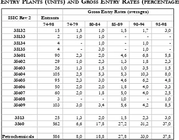
Table 2 reports information on gross entry (NE_i) for each of the thirteen petrochemical in-dustry groups. There were 586 plant start-ups during the 25 years span and entry was concen-trated in plastics, reflecting the fact that this group of industries requires less amount of capital investment and that the technology to enter is standardized. The entry rate exhibits an increase in plastics and remains constant within resins. There is not enough information to compare the data with that found in international studies.7

Three additional comments are necessary. First, Gross entry in plastics was concentrated in three sub-industries. They were the manufacture of tubular films and synthetic guts, the manu-facture of furniture and plastic products not classified elsewhere and the manumanu-facture of basic plastic shapes, sheets, films and tubing. Almost 300 start-ups took place in them. These are

industries with strong links to packing and housing that performed relatively well during all the period. Second, overall entry in the petrochemical industry does not appear to be cyclical. Ex-ception made for initial years (1974-79) and the years 1990-91, the number of firms entering the market was quite even and not dependent of the overall business cycle. For instance, in the first years of the 1980’s, the Colombian economy suffered a slowdown in its economic growth but the number of entrants kept its pace.

Third, it is worthwhile comparing the period 1974-89 with the period 1990-98. The ratio-nale is that during the first period there was a standing policy to protect national industry from foreign competition. The data seems to confirm the hypothesis that plant entry was boosted after the economic liberalization of 1991. The annual number of start-ups was 35 between during the decade against the average of 18 startups between 1974 and 1989.

T

2

E

P

(

)

G

E

R

(

)

Source: Own estimations based on DANE-EAM

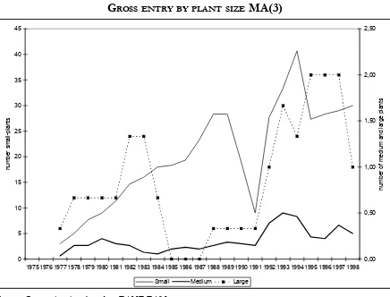
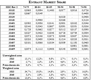
Figure 1 illustrates gross entry by plant size for overall the period. The main feature is that the larger proportion of firms entering the industries was composed of small and medium size plants.8 _{After 1994 entry flows apparently recovered. Table 3 summarizes the measures of} penetration rates. The measures indicate low penetration rates. The long run average for the entire industry is 6.8% when rates are weighted by plant output market share. The plastic industry exhibit rates, where on average entrants explain 5% of its group output. In resins

Gross Entry Rates (averages) ISIC Rev 2 Entrants

74-98 74-79 80-84 85-89 90-94 95-98

35132 15 1,5 1,0 1,5 1,7 3,0

35133 2 1,0 1,0 - -

-35134 4 - 1,0 - 1,0

-35135 4 - 3,0 - 1,0

-35601 90 2,3 2,0 4,6 6,8 5,8

35602 29 1,0 2,3 1,3 1,8 2,3

35603 26 1,3 1,5 1,0 3,5 1,5

35604 105 2,5 5,3 5,3 10,3 8,0

35605 95 2,3 3,0 4,6 6,2 4,8

35606 50 2,0 2,0 1,8 4,0 3,3

35607 60 2,0 1,8 5,0 4,0 2,5

35608 3 - - 1,0 - 1,0

35609 103 3,0 3,4 5,6 4,2 8,5

3513 25 1,3 2,0 1,5 2,3 3,0

3560 562 6,6 17,8 27,2 31,2 37,0

Petrochemicals 586 8,0 18,8 27,8 33,0 37,8

despite the lower entry rates new plants explain 16% of its sector output. These numbers are consistent with findings of other studies on firm entry. For instance, Cable & Schwalbach (1991) reports penetration rates for seven OECD countries and Korea across manufacturing groups covering different periods in the 70s and 80s. For the chemical industry Portugal has a 33% penetration rate, followed by the US with a rate of 19%.

F

1

G

MA(3)

Source: Own estimations based on DANE-EAM

For the remaining cases, entry penetration rates range for 1.5% to 6%. Therefore, one can claim that the first stylized fact applies to the petrochemical industry. Gross entry is a common economic force, averaging 24 firms during 1974-1998, and entry rates are larger than penetration rates.

Survival and post-entry performance of entering plants is another feature that character-izes entry patterns within an industry. Figure 2 shows the evolution of survival rates with plant ageing. Complementary information concerning survival by cohorts is in Appendix I. The figure was reached by summing up the number of firms that survive across each cohort, and dividing it by the total number of entrants. It is clear that as firms age their survival likelihood declines. Some facts can be noticed. First, a very low number of firms/plant die during the first two years of birth, meaning that new firms adopt tough competition strategies. The average life span of new firms is high. It takes about seven years to get a survival indicator of less than 50%. Mata (1995) shows a figure of the survival schedule of new plants in Portugal. The shape

0 5 10 15 20 25 30 35 40 45

1975 1976 1977 1978 1979 1980 1981 1982 1983 1984 1985 1986 1987 1988 1989 1990 1991 1992 1993 1994 1995 1996 1997 1998

num

ber sm

al

l-pl

ant

s

0,00 0,50 1,00 1,50 2,00 2,50

num

ber

of

m

edi

um

and

l

a

rge

pl

ant

s

of the function is convex, which implies an increasing rate of firm deaths. In a similar way, the shape of the function for the samples of Colombian petrochemicals firms is also convex, im-plying the same behavior.9

T

3

E

M

S

ISIC Rev 2 74-79 80-84 85-89 90-94 95-98 74-98 35132 0,0865 0,0094 0,1480 0,0577 0,0016 0,0726

35133 0,8667 0,0149 . . . 0,4408

35134 . . . 0,0320 . 0,0408

35135 . 0,9980 . 0,0268 . 0,5124

35601 0,0582 0,0056 0,0141 0,0801 0,0332 0,0346

35602 0,0143 0,0343 0,0607 0,0091 0,0351 0,0336

35603 0,1728 0,0662 0,0277 0,0112 0,0137 0,0590

35604 0,0237 0,0423 0,0248 0,0728 0,0784 0,0504

35605 0,0573 0,0146 0,0375 0,0440 0,0657 0,0416

35606 0,0233 0,0400 0,0456 0,1214 0,0235 0,0531

35607 0,0181 0,0066 0,0184 0,0559 0,1193 0,0465

35608 . . . . 0,0801 0,0801

35609 0,0874 0,1112 0,0408 0,0145 0,0902 0,0641

Unweighted rates

3513 13,1% 12,2% 9,0% 2,7% 0,1% 8,1%

3560 2,7% 2,3% 2,5% 4,6% 5,3% 3,4%

Petrochemicals 5,3% 4,7% 3,1% 3,5% 3,3% 4,0%

Weighted rates

3513 34,7% 19,5% 14,8% 3,9% 0,2% 16,0%

3560 5,3% 3,9% 3,3% 4,5% 5,8% 4,5%

Petrochemicals 13,6% 6,1% 4,0% 4,6% 5,6% 6,8%

9 _{Two caveats are important to have in mind. Since we ruled out all firms that did not report information for at least}

four years, many small starts-up that fell into that classification actually could have survived and so the survival indicator may be understated. Second, the percentage of firms surviving more than fifteen years may be under-stated given the changes in the ID code number and the high gross exit that occurred in 1991 and 1992.

Source: Own estimations based on DANE-EAM

Methodology: Entrant Market Share (Penetration rate): ESH(t) = QE(t)/QT(t)

0,00 0,10 0,20 0,30 0,40 0,50 0,60 0,70 0,80 0,90 1,00

1 2 3 4 5 6 7 8 9 10 11 12 13 14 15 16 17 18 19 20

years

share

The survival of medium size plants is longer as expected. Indeed they had a remarkable consistency and resiliency. On average, their survival rate was greater than 90% per cent for all cohorts. On the other hand, small-size plants face more trouble trying to survive as can be noted from their consistently lower proportion within plant population ageing.

In sum the highlighted entry patterns indicate that the results fit along the expected direc-tion and magnitudes, relative to what other studies have found within the chemical industry. Thus, the gross entry penetration rates are low. The analyzed sample gives no evidence of the existence of either entry or exit waves (shake-out). Firm survival indicates that the medium-size plants accommodate to post-entry competition exhibiting the highest survival rates. The petrochemical industry as a whole tends to reduce plan size over time, which gives firms more flexibility for plant restructuring. The next section turns attention to productivity analysis by entry dynamics.

F

2

P

0,00 0,20 0,40 0,60 0,80 1,00

1 2 3 4 5 6 7 8 9 10 11 12 13 14 15 16 17 18 19

years

Small Medium Large

F

3

S

Source: Own estimations based on DANE-EAM

III. P

This section presents the results of measuring productivity and technical change within a panel of industrial plants that belong to the plastics and synthetic resins industries. These spe-cific groups form the petrochemical sector in Colombia as depicted by diagram1. The exercise looks to establish whether there are productivity differentials across type of firms according to their entry status and asks the question of whether entrants do better than incumbent firms within the market. The section is divided in three parts. It begins presenting the methodology for measuring total factor productivity following the Divisia index approach. Then it turns to specific data issues on the format of the longitudinal dataset, and finishes presenting an analy-sis of sources of productivity growth.

3.1 T

production functions. By far the most used in productivity studies [Jorgenson et. al (1987)] is the translog index of TFP growth, also known as the Tornqvist-Theil index. The technology behind such index is the transcendental logarithmic production function [Christensen et. al. (1971)] restricted to constant returns to scale. A common refinement to the Tornqvist index is to take into account the effects of changes in quality in inputs [Jorgenson and Griliches (1967)], in which aggregate inputs follow a translog specification in each one of its components.

The translog index has some desired economic properties such as being an exact transfor-mation of a translog production technology. The index is also time-chained, which allows fac-tor shares to change over time. This feature makes it unnecessary to assume neutrality in technical progress under the hypothesis of perfect competition. Changes in input value shares will be the result of changes in factor marginal rates of substitution.10 _{The Translog index of TFP growth} for any given firm is

1 1

1

1 1

1

ln ( ) (ln ln )

2

n

t t

it it it it i

t t

A Y

Ln S S x x

A− Y− = − −

= − ⋅

∑

where: s_i = factor i’s share in gross output at time t; x_i = type of input i; A_t = Hicks-neutral index of technical change at time t; and Y_t = firm gross output at time t.

It follows that under the classical assumptions the rate of growth of TFP is equivalent to the rate of technical progress. The underlying technology of (11) is the restricted Translog production function under constant returns to scale. The used translog function includes four types of inputs for every industry sector i: capital, labor, materials, and energy. Let

( , , , )

i i i i i i

Y = A F K L M E⋅ (12)

denotes firm i’s production function, and

2

0 i i ij i j t tt it i

i i j i

1 1

ln Y(X, t) b b ln x b ln x ln x b t b t b t ln x

2 2

= +

∑

∑∑

∑

be the translog specification of (12), where X and t denote the vector of inputs and time argument respectively. Factor elasticities in (13) are equal to

i

x i ij j iT

j i

ln Y

V b b ln x b t

ln x

∂

= = + +

∂

∑

On the other hand, the rate of technical change is equal to the growth of output holding all inputs constant, which is given by

T T Tj j TT

j

ln Y

V b b ln x b t t

∂ _{= = + +}

∂

∑

10 _{The observed changes in factor shares are explained also by changes in factor prices that are not related to changes}

Necessary conditions for producer equilibrium imply that factor elasticities are equal to the value shares of inputs in gross output if the technology exhibits constant returns to scale (CRTS), and inputs are paid by their marginal products. Since the production function (13) is assumed linearly homogeneous, applying Euler’s theorem implies

n i i i Y x Y x ∂ _{⋅ =} ∂

∑

The above identity is known in production analysis as the adding up condition implying that output is fully accounted by all input payments. To satisfy (16) the value of inputs must sum to 1, hence

xi i ij j it

i i i j i

V = b + b ⋅ln x + ⋅t b

∑

∑

∑∑

∑

i

V =1

∑

For this restriction to apply globally, it follows

i i

b =1

∑

b =0

∑

The translog function can be evaluated to express the growth rate of output as the weighted sum of the growth rates in inputs plus the rate of productivity growth in two discrete points in time,11 _as

[

]

1 1

ln Y(T) ln Y(T 1) V V [ln x ln x ] [V V ]

2 − − 2 −

− − = ⋅

∑

Finally, if restrictions (18) are imposed on the above growth decomposition equation, factor elasticities are equivalent to input shares, and Eq. (19) becomes the translog index given by formula (11). In other words, this index represents the rate of technical change for a plant i, when the current technology can be approximated by a translog production function. Regarding input capital, labor, and materials, they also follow a translog specification on their compo-nents. Under the assumption of CRTS, the translog index for each input i becomes

n t

jt jt 1 jt jt 1 j 1

t 1

K 1

Ln ( ) (ln k ln k )

K− 2 = − −

= ⋅

∑

n t

jt jt 1 jt jt 1 j 1

t 1

L 1

Ln ( ) (ln l ln l )

L− 2 = − −

= ⋅

∑

n t

jt jt 1 jt jt 1 j 1

t 1

M 1

Ln ( ) (ln m ln m )

M− 2 = − −

= ⋅

∑

11 _{Because the translog function is a special case of the generalized quadratic function, using the quadratic}

where θ_j denotes the share of each component in input’s total payments. Equations (20) to (22) express the growth rate of aggregate capital, labor, and materials by the sum of growth rates of each sub-input weighted by its average marginal product, under the assumption input and out-put competitive markets. The weighted sum among inout-puts represents the correction by improve-ments in the quality of inputs that are embodied in the process of technical change itself. 12 _Thus, formulas (11) and (11)-(22) constitute the benchmark for measuring total factor productivity across plants in our study panel.

3.2 D

The analysis of plant productivity is based on a longitudinal dataset that includes all plants that report consistently at the Colombia’s Annual Manufacturing Survey [Encuesta Anual Manufacturera (EAM)] for the 1975-1998 period. There were 921 identified plants that at some point have records at the survey within the plastic and synthetic resins sectors. Nonetheless, 298 plants were dropped form the panel for several data inconsistencies and then were classi-fied as volatiles. The exclusion of those plants reduces the number of plants to 623 in the working panel. This final panel is slightly different from the one used in section II to measure entry and exit rates. The objective here is to work with individuals that have consistent records in the basic variables of output, investment, labor input, materials and power consumption that allow to get accurate measures of input demands and total factor productivity.13

The EAM until 1977 published the variable of plant startup year. Later we consider as the startup year the first record that shows up in the panel. The exit date is the year by which there are no records afterwards. Therefore, plants were classified according to entry dynamics. Incumbents are plants that show records for the entire period, entrants are surviving plants that begun operations after 1977 and are still active in 1998, and the existing plants are those founded before 1977 or entrants after 1977 that exit the market before 1998.

Table 4 depicts the average number of industrial plants and the average plant output, capital stock, and employment within the petrochemical industry by five-year periods. There are several plant characteristics worth to highlight. To begin with there is a notorious difference in capital intensity between the two industry branches. On average, the capital stock per plant in synthetic resins moved 6.3 in the 70s to 14.2 times at the end of the 1990s. Plant size is on average 3.5 times larger in resins, given by the number of employees. In both cases plant size started decreasing since 1990 in both sectors. This adjustment suggests labor restructuring

12 _{Among many studies on productivity, this correction has been applied in the works of Jorgenson et al, (1987) for}

the U. S, and Young A., (1994) for East Asian countries. An application for the manufacturing sector in Colombia is in Pombo (1999a).

13 _{The plants in the panel fulfill the following requirements in order of not being classified as volatile plants: i) plants}

14 _{See Pombo & Ramirez (2003) for further details.}

within plants to minimal efficiency scales. The above differences also hold for type of plants according to entry dynamics. Incumbents tend to use more capital-intensive technologies and plants are larger in size and in their operative scale. On average, plant output for incumbent plants is 2.5 times larger than for entering plants. In contrasts, exiting plants show decreasing patterns in their characteristic variables.

3.3 S

The first step in analyzing productivity and market entry is to answer two basic questions: i) How is the performance of total factor productivity across plants by type entry dynamics? That is, do entrants perform better than incumbents?, and does productivity slowdown influence market exit, and ii) if so, does productivity drive output growth?

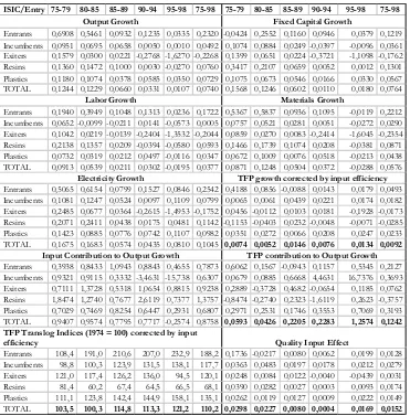
Total factor productivity is measured using translog indices given by Eq. (11). Positive changes in those indices reflect productivity gains due to technical change. Table 5 synthesizes the results about the measurement of the sources of growth, the contribution of technical efficiency to output growth, and the quality input effect. The measurement of TFP was done for all 623 plants of the panel. Afterwards inputs and output variables were weighted and grouped according to ISIC-specific group within the synthetic resins and plastic industries and market entry dynamics. That is plants/firms were coded as surviving entrants, incumbents and exiting firms. Then the translog decomposition of industry productivity follows.

The first fact worth noticing is that the measurement is consistent with the expected direction in accordance with plant entry. Entrants are more efficient than incumbents and dying plants are the least efficient. In particular, productivity grew at an average rate of 4.9% per year within entrants, incumbents at 1.8%, while dying plants showed a negative rate of -1.7% per year during the 1975-1998 period.

T

4

P

:

Source: Own estimation based on DANE-EAM;

Notes: ISIC 3513 = Synthetic Resins; ISIC 3560 = Plastics; Petrochemicals = 3513 + 3560; value series are in millions of pesos at 1998 prices.

Entry/ISIC Average Number of plants Average output per plant

classification 74-79 80-84 85-89 90-94 95-98 74-79 80-84 85-89 90-94 95-98

Entrants 4 46 115 228 367 2.049 7.698 5.791 5.216 5.082

Incumbents 74 78 78 78 78 5.456 8.142 12.460 12.996 14.654

Exiters 49 76 109 85 15 5.123 4.512 4.059 2.722 1.117

Resins 10 18 21 24 29 25.381 29.960 45.408 44.763 40.860

35132 6 9 11 13 17 23.269 27.212 45.819 44.695 43.715

35133 2 3 3 2 2 40.323 28.084 38.982 26.998 13.086

35134 2 2 3 4 6 21.538 17.009 17.694 12.174 14.219

35135 1 3 4 5 4 744 42.692 69.465 83.818 82.585

Plastics 117 183 282 367 431 3.453 4.366 4.050 3.726 4.256

35601 24 33 51 65 80 7.124 11.917 10.200 7.922 8.113

35602 6 11 16 19 25 1.683 1.959 2.668 3.530 3.163

35603 8 13 13 15 18 1.159 1.790 2.680 5.472 6.681

35604 21 33 51 69 88 2.423 2.716 3.019 2.793 2.862

35605 24 36 52 70 79 2.197 2.723 2.823 3.036 4.025

35606 14 21 23 30 38 1.840 1.966 2.524 3.737 3.876

35607 4 10 27 35 34 13.177 8.352 3.438 850 1.087

35608 1 3 896 1.370 954

35609 15 28 48 62 66 1.660 1.978 2.179 2.442 3.489

Petrochemicals 127 200 302 391 460 5.198 6.618 6.863 6.276 6.587

Average capital stock Average number of employees per plant

Entrants 4.312 3.989 2.276 2.232 1.703 45 72 54 52 48

Incumbents 2.060 3.442 4.266 4.056 4.260 82 88 80 84 80

Exiters 1.339 1.361 1.157 708 370 102 86 61 40 23

Resins 8.170 14.946 18.699 19.809 16.177 164 231 240 199 124

35132 9.599 18.251 20.785 21.117 16.042 124 143 135 118 85

35133 7.891 8.978 12.171 7.866 3.982 375 295 345 215 105

35134 5.827 5.412 3.757 2.254 3.372 105 97 83 59 42

35135 122 16.754 29.699 38.948 42.026 25 442 554 540 428

Plastics 1.281 1.525 1.187 1.096 1.136 82 70 50 47 48

35601 2.527 4.196 2.973 2.837 2.894 106 95 64 58 51

35602 195 198 188 263 199 43 38 29 37 30

35603 677 783 1.880 1.946 1.942 48 53 48 64 65

35604 981 804 696 700 550 55 44 36 39 36

35605 1.219 1.478 1.028 1.041 1.162 71 60 50 50 61

35606 427 443 523 608 606 49 48 39 55 55

35607 4.349 2.586 1.279 429 232 406 254 104 33 28

35608 211 360 260 24 33 21

35609 448 517 525 457 704 71 55 42 43 55

Petrochemicals 1.836 2.710 2.388 2.257 2.093 89 84 63 56 53

The analysis of sources of growth shows that the petrochemical industry had a modest rate of TFP growth. The long rung growth rate is 0.92%, which is similar to rates estimated in other studies for total manufacturing that is around 0.8% per year.15 _{Output growth in petrochemicals} was sustained by capital accumulation up to 1985 where capital stock rate of growth is 14% per year. Then there was a drastic slowdown in capital accumulation. The average rate during the 1990s dropped to 1.5% per year. The contribution of TFP to output growth in contrast increased

15 _{For more details see Pombo (1999b). The estimates of this study are based on ISIC 4-digits groups and do not}

since 1985. Technical change arose as source of output growth during the 1090s. The contribu-tion of TFP to output growth was 74% while the reminder 16% were allocated among inputs. This scenario was opposite in the 1970s where inputs contributed 94% to output growth.

There are at least three facts worth mentioning if one breaks the industry by entry dynamics. First, industry growth is based on the entry flows. This fact is clear in plastics where entry rates steadily increased over time [Table 1]. Entrants as defined for this exercise are surviving plants that enter in the market after 1977. This implies that the first cohorts of those firms after 20 years became the dominant ones in the industry. In fact, entrants ended up demanding more capital or labor inputs. Thus, younger firms gain over time market share and generated more employment. This implies a positive trend of birth cohorts where new firms shape the industry in the long run.

T

5

S

, TFP

, Q

AND INDUSTRYGROUPS

Methodology: Input quality effect = TFP growth corrected - TFP growth simple Source: Own Estimations based on DANE-EAM

ISIC/Entry 75-79 80-85 85-89 90-94 95-98 75-98 75-79 80-85 85-89 90-94 95-98 75-98

Output Growth Fixed Capital Growth

Entrants 0,6908 0,5461 0,0932 0,1235 0,0335 0,2320 -0,0424 0,2552 0,1160 0,0946 0,0379 0,1219

Incumbents 0,0951 0,0695 0,0658 0,0050 0,0010 0,0492 0,1074 0,0884 0,0249 -0,0397 -0,0096 0,0361

Exiters 0,1579 0,0300 0,0221 -0,2768 -1,6270 -0,2268 0,1399 0,0651 0,0224 -0,3721 -1,1098 -0,1762

Resins 0,1360 0,1472 0,1000 0,0030 -0,0270 0,0760 0,3417 0,2107 0,0659 0,0052 0,0012 0,1301

Plastics 0,1180 0,1074 0,0378 0,0585 0,0350 0,0729 0,1075 0,0673 0,0546 0,0166 0,0330 0,0567

TOTAL 0,1244 0,1229 0,0660 0,0331 0,0107 0,0740 0,1568 0,1246 0,0602 0,0110 0,0180 0,0764

Labor Growth Materials Growth

Entrants 0,1940 0,3949 0,1048 0,1313 0,0236 0,1722 0,5367 0,5837 0,0936 0,1095 -0,0119 0,2212

Incumbents 0,0652 -0,0099 -0,0211 0,0141 -0,0573 0,0005 0,0757 0,0521 0,0281 0,0051 -0,0272 0,0290

Exiters 0,1042 0,0219 -0,0139 -0,2404 -1,3532 -0,2044 0,0859 0,0270 0,0083 -0,2414 -1,6045 -0,2354

Resins 0,2138 0,1357 0,0209 -0,0394 -0,0580 0,0593 0,1466 0,1739 0,1074 0,0208 -0,0381 0,0871

Plastics 0,0732 0,0319 0,0212 0,0497 -0,0116 0,0347 0,0672 0,1009 0,0076 0,0518 -0,0213 0,0438

TOTAL 0,0913 0,0539 0,0211 0,0302 -0,0195 0,0377 0,0871 0,1248 0,0504 0,0372 -0,0288 0,0576

Electricity Growth TFP growth corrected by input efficiency

Entrants 0,5065 0,6154 0,0799 0,1527 0,0846 0,2542 0,4188 0,0856 -0,0088 0,0143 0,0179 0,0493

Incumbents 0,1081 0,1247 0,0524 0,0097 0,1109 0,0799 0,0065 0,0061 0,0439 0,0221 0,0174 0,0182

Exiters 0,2485 0,0677 0,0364 -0,2615 -1,4953 -0,1752 0,0456 -0,0112 0,0103 0,0181 -0,1928 -0,0173

Resins 0,2071 0,2411 0,0438 0,0175 0,0481 0,1142 -0,1153 -0,0403 0,0232 -0,0048 -0,0071 -0,0285

Plastics 0,1423 0,0885 0,0776 0,0742 0,1107 0,0982 0,0351 0,0272 0,0066 0,0208 0,0247 0,0233

TOTAL 0,1675 0,1683 0,0574 0,0435 0,0810 0,1045 0,0074 0,0052 0,0146 0,0076 0,0134 0,0092

Input Contribution to Output Growth TFP contribution to Output Growth

Entrants 0,3938 0,8433 1,0943 0,8843 0,4655 0,7873 0,6062 0,1567 -0,0943 0,1157 0,5345 0,2127

Incumbents 0,9321 0,9115 0,3332 -3,4631 -15,738 0,6307 0,0679 0,0885 0,6668 4,4631 16,7376 0,3693

Exiters 0,7111 1,3728 0,5318 1,0654 0,8815 0,9238 0,2889 -0,3728 0,4682 -0,0654 0,1185 0,0762

Resins 1,8474 1,2740 0,7677 2,6119 0,7377 1,3757 -0,8474 -0,2740 0,2323 -1,6119 0,2623 -0,3757

Plastics 0,7029 0,7469 0,8254 0,6447 0,2931 0,6807 0,2971 0,2531 0,1746 0,3553 0,7069 0,3193

TOTAL 0,9407 0,9574 0,7795 0,7717 -0,2574 0,8758 0,0593 0,0426 0,2205 0,2283 1,2574 0,1242

TFP Translog Indices (1974 = 100) corrected by input

efficiency Quality Input Effect

Entrants 108,4 191,0 210,6 207,0 232,9 188,2 0,1736 -0,0217 0,0080 0,0062 0,0199 0,0128

Incumbents 98,8 100,3 123,9 131,5 138,1 117,7 0,0363 0,0483 0,0197 0,0178 0,0212 0,0279

Exiters 121,0 117,4 126,2 136,0 94,5 120,1 0,0248 0,0084 0,0122 -0,0040 -0,0439 0,0031

Resins 81,4 60,2 67,4 64,5 66,5 68,1 0,0390 0,0282 0,0027 0,0003 0,0093 0,0174

Plastics 111,1 123,8 142,4 144,9 158,1 135,1 0,0262 0,0119 0,0127 0,0009 0,0222 0,0149

F

4

T

I

TFP (1974=100) - C

. P

I

20 40 60 80 100 120 140 160 180

1970 1972 1974 1976 1978 1980 1982 1984 1986 1988 1990 1992 1994 1996 1998

TFP

-I

n

d

ic

e

s

ISIC3513 ISIC3560 ISIC35

F

5

T

I

TFP (1974=100) - P

.

M

80 85 90 95 100 105 110 115 120 125 130

1970 1972 1974 1976 1978 1980 1982 1984 1986 1988 1990 1992 1994 1996 1998

TFP

-I

n

d

ic

e

s

petrochemical manufacturing

Second, there is a catching-up in productivity growth between the surviving entrants and incumbents according to the table. The first cohorts were on average highly productive. TFP growth was on average 42% per year in the late 1970s and 8.5% during the first half of the 1980s. The catching up of TFP growth is evident for the late 1990s where either entrants or incumbents plants had on average 1.7% productivity growth. Third, incumbent firms accom-modated to market entry. TFP contribution to output growth is higher than input contribu-tion among entrants for the first cohorts, but this was not the case after 1980. The numbers for incumbent firms suggest that the loss in market share with respect to entrants induced plant restructuring since the mid 1980s. TFP growth confirms partly this observation. The average rate for the second half of the 1980s was 4.4% and 2.2% for the first years of the 1990s. Entrants showed no productivity growth during the late 1980s and 1.4% in the early 1990s. The demand for capital input was drastically reduced after 1985. The annual accumu-lation rate moved from 8.8% to 2.5% in the 1980s. After 1990 it turned negative. Entrants in contrast kept positive growth rates in their capital stock, although they exhibit a decreasing trend over time.

The demand for labor input across incumbents was on average negative since 1980, reach-ing a minimum of –5.7% for the second half of the 1990s. In contrast, entrants displayed a 17% long run rate in labor input. The above numbers, together with the null growth in output for incumbent plants during the 1990s, imply an outlier TFP contribution to output growth of 4.4 and 16.7 times offsetting the drastic reduction of aggregate inputs contribution to growth. Intermediate consumption gathers the demand for raw materials, and the consumption of fu-els, lubricants, repairing services, and machinery parts. Electricity demand is excluded because it is treated separately as an input.

Savings in materials spending is a source of efficiency gains. Consumption growth in inter-mediate materials decreased for incumbents as well as for entering plants since the late 1970’s. Nonetheless, efforts on saving in material spending were very evident for entrants. They could diminish by 48 percentage points the spending in intermediate materials, moving from 58% to 10% growth rates from 1980 to 1994. For the same period incumbents, reduced them in 4.7% moving from 5.2% to 0.5% annual growth rate. Technical change became a source of growth within plastics since the mid-1980s when entry within this industry took off.

Last, the change in quality of inputs is an important source of productivity gains in this industry. On average, there is a difference of 1.5% TFP growth per year. This effect is impor-tant within all subgroups in the petrochemical industry. The difference in resins is 1.7% while in plastics is on average 1.5% per year in TFP growth.

IV. P

The main shortcoming of following an index approach methodology to measure techni-cal change and total factor productivity is that it does not account for the effect of market entry and exit in industry productivity. Firm entry is an endogenous flow that shifts either plant or industry-group productivity. The literature on index numbers and productivity measurement has developed methodologies since the 1970s relaxing the core assumptions that are behind the traditional TFP decompositions.16

The analysis of plant turnover has attracted attention within the productivity literature in recent years because economies around the world have engaged in a series of structural market reforms that have implied market deregulation, elimination of entry barriers and promotion of market competition since the 1990s. Firm entry has an effect on plant reallocation and shakeout of inefficient firms. These effects in fact might induce plant restructuring. Thus, entry and exit flows force firms to become more productive over time in order to survive. Enterprises that cannot make it fail end exit the market.17 _{The non-parametric estimation of a given industry group} productivity index level can be defined as the weighted sum of firm productivity level at year t:

t it it

i 1,n

LnTFP ln TFP

=

=

∑

where i indices plants, TFP is the translog index derived from Eq. (11), and θ it is plant weight

in industry-ISIC specific gross output. This formulation is interesting from the view of output reallocation across firms. In particular, if high productivity firms gain participation this will contribute positively to industry productivity growth even if no individual firm experiences a productivity increase. Following Olley & Pakes (1996), given any particular estimation of plant productivity levels, Eq. (23) decomposes in two terms:

1 6 _{On this particular, productivity studies at firm or industry levels have introduced market failures and measured}

TFP through the inclusion of markups and imperfect competition [Hall (1988)], output scale [Nadiri & Schankerman (1981)], rate of return of regulation [Denny, Fuss, & Waverman (1981)], factor demand endogeneity and quasi-fixed inputs [Morrison (1986, 1988, 1992)], rate of installed capacity utilization [Fuss & Berndt (1986)], and entry, exit and turnovers [Olley & Pakes (1996), Griliches & Regev (1995), and Foster, Hatinwanger & Krisan (2001)]. For the case of Colombia a non-parametric measurement of TFP introducing imperfect competition through mark-ups and variable returns to scale for ISIC-group in manufacturing is in Pombo (1999b).

17 _{Melendez et al (2003) presents a TFP parametric estimation at plant level and groping results at 2-digits ISIC}

18 _{We follow the notation used in the study of Aw, Cheng, & Roberts (2001).}

N

t it t t it t

i 1

LnTFP [ ( )][ln TFP (ln TFP ln TFP )

=

=

∑

t N t

t t it it

i 1

LnTFP N ln TFP ln TFP

=

= θ ⋅ +

∑

hence,

t N

t _{it it}

i 1

LnTFP ln TFP ln TFP

=

= +

∑

where ln TFP_t is the mean productivity over all plants in year t and θ_tis the plant share in year t. The second term of Eq. (24) represents the sample covariance between plant productivity and output. It follows that the larger the covariance is, the larger the share of more productive plants and therefore the higher industry-group productivity will be.

An alternative TFP decomposition focuses on the measurement of productivity growth ac-cording to entry dynamics following Griliches & Regev (1995). This decomposition defines the contributions of continuing firms, the difference in average between entering and exiting co-horts and reallocation of market shares into the TFP residual among all plants. In particular, if high productivity firms gain participation this will contribute positively to industry productivity growth even if no individual firm experiences a productivity increase. Taking differences of (13) one can express changes in productivity over time for a single plant i as

(

)

(

)

t t 1

t 1 t 1 t t t 1 t

t 1 t

t 1 t

ln TFP ln TFP ln TFP ln TFP

2

ln TFP ln TFP 2

+

+ + +

+

+

θ + θ

 

θ − θ =_{ }⋅ −

 

+

 

+_{ } θ − θ

 

(25)

Eq. (25) says that the contribution of plant i to an industry productivity growth is the sum of two components: i) the weighted own productivity growth by market share, and ii) the change in its market share weighted its productivity average. If there is no entry or exit at time t and t+1, this implies that industry productivity will equal the sum of productivities over all plants given Eq. (4). An increase in market reallocation from low productivity to high produc-tivity firms and/or a single firm producproduc-tivity increase will explain industry producproduc-tivity growth under this decomposition. Now, if entry or exit occurs the above-mentioned set up is not longer useful. The shortcut that Griliches & Regev (1995) proposed is to aggregate in a given two-year period all entrants (E) at year t+1 and all dying plants (D) at year t as a single firm with weight in output or sales θE t,+1 and θD t, respectively. Aggregating over continuing firms and adding

(

)

(

)

(

)

(

)

it

D,t E,t 1 it i,t 1

E,t 1 D,t i,t 1

i 1,n

E,t 1 D,t it i,t 1

E,t 1 D,t i,t 1 it

i 1,n

ln TFP ln TFP ln TFP ln TFP ln TFP

2 2

ln TFP ln TFP ln TFP ln TFP

2 2

+ +

+ +

=

+ +

+ +

=

 

θ + θ θ + θ

   

∆ =_{ }⋅ − + _{ }⋅ − _

    

 

+ +

   

+_{ }⋅ θ − θ + _{ } θ − θ _

    

∑

∑

The above formula decomposes an industry ISIC-group productivity growth in four parts: i) the turnover effect between entrants and dying firms, ii) the contribution of continuing plants, iii) the market share reallocation among entrants and existing firms, and iv) the market share reallocation from low to high productivity of continuing firms. The last two terms can be simply added to denote market share reallocation effect.

4.2 P

D

Market entry influences industry cycles, restructuring processes, and transitions. This sec-tion presents a comparative analysis of productivity differentials between entering, incum-bents, and dying plants, and across birth cohorts with the purpose of shedding light at the role of entrants in industry productivity. The goal is therefore to determine if productivity differen-tials reveal turnover patterns. The working panel, as mentioned, has a total of 623 petrochemi-cal plants distributed between plastics and synthetic resins. The older plant in the panel started operations in 1933 and the younger ones did in 1995. Because we are working with continuous information since 1974 it was necessary to classify plants according to birth cohorts by five-year periods to simplify the analysis.

Diagram 2 draws the map of industrial plants based on the five-year period, entry cohort and transition status. There are five working cohorts from 1975 to 1998. The chart flow has five layers indicating what the plant cohorts are. Plants might belong to cohorts a, b, c, d, and z. Each cohort has assigned a subscript of five-year period. Thus plants belonging to the first cohort (a) are those plants founded before 1979. They split in two groups. The surviving plants that report data for the next period, and the dying plants that exit the market during the period. They are marked with the superscript S and X respectively. The second layer indicates the plants that were born between 1980 and 1984. Thus the staked data in the panel within this period have records from plants from the first and second cohorts (a and b). Again plants might survive or exit the market regardless their cohort. Surviving plants from the cohorts (a) and (b) will have records in the next period [1985-1989]. At the same time new plants enter in the market within the period and are grouped as cohort (c). The reading of the entry and exit flows continues in the same manner up to the last cohort/period, which has plants from all five cohorts.

F IRM E NTR Y , P R ODUCTIVITY D IFFERENTIALS AND T URNO VERS IN I MPORT S UBSTITUTING M ARKETS

Borradores de investigación - No. 42

of testing changes in means and medians. These tests depict the direction that a firm perfor-mance variable such as productivity takes within a given sample. The test on medians evaluates proxy distribution shape through the non-parametric Wilcoxon rank-sum test.19

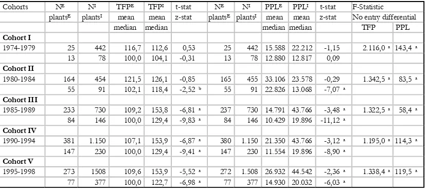
Table 6 summarizes the results of this exercise. The sample size (N) is equal to plant-year observations according to birth cohort. Incumbents are individuals that report for the entire pe-riod, entrants are successful births for any given period that are still active by 1998, and exiting plants are those that shut down operations within a given period. Thus, incumbents and entrants in this context form the surviving plants.20 _{Differences in total productivity levels given by the} TFP translog indices are statistically significant at 1 percent level for the first three cohorts. The mean (median) difference between surviving and exiting plants is 17 (11.5) points for cohort I, 42 (13.2) points for cohort II, and 26 (6.3) for cohort III. In contrast, for cohort IV we cannot reject the hypothesis of no productivity differentials. The outcomes for labor productivity are robust and go in the same direction. On average labor productivity is higher in surviving plants but the difference tends to close over time. For instance the mean (median) is $26.9 ($7.1) millions per worker/year for cohort I, $8.4 ($2.6) millions for cohort II, and $2.8 ($2.3) millions for cohort III. The mean labor productivity differential for cohort IV raises but not its median, which remains almost constant ($2.9 millions).21 _{The differences are significant at 5% level.}

The second implication of the firm selection model further restricts the test on productivity differentials. In particular, if surviving firms are in fact more efficient over time, is there a difference between incumbents and successful entrants? TFP growth showed a long run rate of 5% per year for entrants and 1.9% per year for incumbent plants. From the perspective of entry flows they indicate that a successful entrant at time t becomes an incumbent firm at time t+1. Then with time passing older entrants’ productivity first catch up with industry benchmarks and then turn into newly incumbents. This process characterizes the formation of generations of entrepreneurs. In the case of petrochemicals in Colombia it is clear that the industry entry patterns indicate that at least two generations of entrepreneurs were created. The older incum-bents that started up from the 1950s to the 1970s and the successful entrants after 1980 lo-cated mainly within the plastic industry.

Table 7 presents the results of testing productivity differentials between entrants and in-cumbents plants by cohort that takes into account entry dynamics where entrants at period t,

turn out incumbents at period t+1. The sample size (N) consists of plant-year observations where the maximum number of records for each plant within a given cohort/period, are 5

19 _{Wilcoxon’s test has several versions. The one that is implemented in STATA software is the extension of}

Mann-Whitney (1947) about rank sum tests. See Sprent & Smeeton (2001) for further explanation on tests for two independent samples.

20 _{For instance, the table report 2195 plants for cohort I. Among them there are plants founded since 1933 up to}

1979. Plants founded in 1978 or 1979 that are still reporting by 1998 are the entrants of this cohort. Plants that report from or before 1977 to 1998 are the incumbents. Exiting plants are the units that fail within the 1974-1979 period. Recall that in all cases the first observation is 1974. The total number of surviving plants of this cohort are 91 while dying plants are 61.

21 _{Notice that there is not exiting plants for cohort V. This is a result of the truncation derived from the conditions}

T

6

P

BY COHORT

P

W

R

-S

T

Notes: X= exiting plants; S=surviving plants. TFP is the translog index of TFP where entry date = 100, PPL = PPL= VA/L, in thousand of pesos at 1998 prices per worker per year. N= Number of observations are firm-year observa-tions. The panel is an unbalanced time series-cross section dataset. Plants= Number of plants or individuals within the panel by cohort and entry dynamics; a= statistically significant at 0.01; b= statistically significant at 0.05; c= statistically significant at 0.1; DUM1= dummy variable to test changes in average TFP and labor productivity between exiting and surviving plants by cohort. The variable takes the value of 1 if marked as an exiting plant. They can be either former incumbents for the first cohort or entrants in successors cohorts. Survival firms are plants, which are successful entrants or survival incumbents. Incumbents in the study are defined as reporting plants for the 1974-1998 period. Methodology: t-tests = Ho: mean(x)-mean(s) =difference=0; z-test= Ho: median(x)=median(s)

Cohorts NX

plantsX

NS

plantsS

TFPX

mean median

TFPS

mean median

t-stat z-stat

NX

plantsX

NS

plantsS

PPLX

mean median

PPLS

mean median

t-stat z-stat

Cohort I

1974-1979 903 2.195 126,1 143,1 -5,47a _{902 2.196 22.561 49.533 -5,85}a

61 91 110,5 122,0 -5,08a _{61 91 15.169 22.270 -10,65}a

Cohort II

1980-1984 391 934 125,9 167,8 -4,97a _{385 935 20.108 28.529 -2,42}a

39 55 109,8 123,1 -5,99a _{39 55 13.000 15.640 -5,39}a

Cohort III

1985-1989 346 989 106,7 132,8 -4,03a _{344 993 19.647 22.451 -1,21}

54 84 100,0 106,3 -4,22a _{54 84 10.923 13.241 -2,64}a

Cohort IV

1995-1998 69 969 125,7 118,0 1,17 69 968 13.762 27.032 -2,04b

15 147 100,1 104,9 -0,70 15 147 10.626 13.516 -2,40b

Cohort V

1995-1998 273 109,6 272 26.932

77 100,0 77 14.930

observations, where the number of incumbents increases over time. It began with 78 plants for cohort I, and ends up with 377 plants in the last cohort. Three results are worth mentioning. First, productivity levels given by the average value across plants of the TFP translog indices follow a concave function reaching a local maximum with an index value of 154 during the 1990-1994 period.