FOOD INFLATION IN BOLIVIA: ITS RELATIONSHIP WITH INTERNATIONAL PRICES AND POLICY RESPONSES Pablo Mendieta Ossio Martín Palmero Pantoja

Paper submitted to XV Central Bank Researchers Network of the Americas

FOOD INFLATION IN BOLIVIA: ITS RELATIONSHIP WITH

INTERNATIONAL PRICES AND POLICY RESPONSES*

Pablo Mendieta Ossio

Martín Palmero Pantoja

* _{This paper is part of a joint research between the World Bank and the Central Bank of Bolivia. The authors}

Food Inflation in Bolivia: Its Relationship with International Prices and Policy

Responses

Pablo Mendieta Ossio and Martín Palmero Pantoja

Keywords: Inflation; Vector-Autoregressive; Small macroeconometric models Clasificación JEL: C32, C5, E3, F0

Abstract:

Between late 2006 and mid 2008, the Bolivian economy experienced a strong rebound in inflation, mainly due to the upturn in external food. This paper discusses the importance of external inflation in the domestic inflation of the Bolivian economy, which is characterized by high dollarization and a crawling peg exchange rate regime For this purpose, we use two alternative methodologies: estimation of a vector autoregressive model (VAR) and a Small Structural Macroeconometric Model (SSMM), which also incorporates the effects on expectations and responses of economic policy, especially monetary and exchange rate policy. The results show that international food inflation played a significant role in the rise of inflation between 2007 and 2008.

Resumen:

Entre finales de 2006 y mediados de 2008 la economía boliviana experimentó un fuerte repunte en la inflación, principalmente debido al incremento de la inflación externa. Este documento discute la importancia de la inflación externa en la inflación en Bolivia, que está caracterizada por alta dolarización y un régimen de tipo de cambio deslizante. Para este propósito, se utilizan dos metodologías alternativas: la estimación de un Vector Autoregresivo (VAR) y de un Modelo Estructural Pequeño (MEP), que incorpora los efectos en las expectativas y las respuestas de política económica, en especial monetaria y cambiaria. Los resultados indican que la inflación internacional tuvo un rol importante en el incremento de la inflación entre 2007 y 2008.

Pablo Mendieta Ossio Banco Central de Bolivia Ayacucho esq. Mercado Telf. (591)-2-2409090 / 2305

pmendieta@bcb.gob.bo

La Paz - Bolivia

Martín Palmero Pantoja

Embassy of United States in Bolivia Av. Arce 2780

Telf. (/591)-2-168986

martinfpalmerop@yahoo.com

I. Motivation

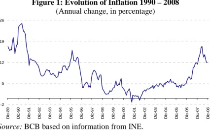
Inflation in the Bolivian economy has been subject to significant fluctuations over the past decades. After the hyperinflationary process in the mid-eighties, when the inflation rate reached record levels, began a process of disinflation that was consolidated in the second half of the nineties and lasted ever since. With the exception of what happened since late 2007, the annual change in the Consumer Price Index (CPI) calculated by the National Statistics Institute (INE) remained below double digits for more than ten years (Cossio et al 2008).

In 2007, inflation started a growing path that lasted until the end of the first half of 2008 when it registered the highest rate in recent years (17,3%). From July 2008 until the end of this year, the inflation rate fell by more than 5 percentage points (pp), to finish the year with an inflation rate of 11,8%, comparable to that registered in 2007, 11,7% (Figure 1).1

Figure 1: Evolution of Inflation 1990 – 2008

(Annual change, in percentage)

-2 5 12 19 26

D

ic

-8

9

D

ic

-9

0

D

ic

-9

1

D

ic

-9

2

D

ic

-9

3

D

ic

-9

4

D

ic

-9

5

D

ic

-9

6

D

ic

-9

7

D

ic

-9

8

D

ic

-9

9

D

ic

-0

0

D

ic

-0

1

D

ic

-0

2

D

ic

-0

3

D

ic

-0

4

D

ic

-0

5

D

ic

-0

6

D

ic

-0

7

D

ic

-0

8

Source: BCB based on information from INE.

The upturn in prices that began towards the end of 2006 has been attributed to several factors that can be broken down into those of internal and external origin. Among those of internal origin are: i) the dynamism of private consumption, due to the good performance of the economy that resulted in better wages and more employment, besides the flow of remittances from abroad, both of which increased the purchasing power of national households; ii) adverse weather events between 2007 and 2008, since Bolivia was hit by El Niño (early 2007), drought (June 2007) and La Niña (late 2007 and early 2008) affecting not only agricultural production but also damaged the road system, hampering the supply of goods to major markets, and iii) an increase in inflationary future expectations of economic agents and market operators that also encouraged price speculation.

1

With regard to external factors, two channels of transmission were detected: dollar depreciation and the rise of international inflation. The first was related to the appreciation of the currencies of the majority of the trading partners of Bolivia, increasing the cost of imports. The second and most important was the increase in commodity prices, especially minerals, fuel and food. This paper discusses the role of international food inflation in the Bolivia economy.

II. Main features of Bolivian food inflation

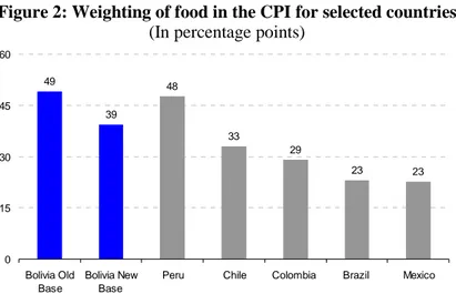
In the case of food’s behavior, they do have consequences on internal inflation. There are two channels: a direct effect via imports of final consumer goods, and indirectly through intermediate inputs for food processing, such as wheat flour, imported input that is essential for making breads, biscuits, and noodles, among the most notable. Additionally, the chapter on greater weight in the basket that makes up the CPI is the chapter of foods and beverages. In fact, is one of the highest in the region, so changes in this division have a strong impact on total inflation.

This is partially due to the weight of the food chapter in Bolivia was one of the highest in the region. Before April 2008, the weighting was 49%, the highest of the countries selected, followed by Peru (48%). Since the change of base, this weight was reduced to 39% (Figure 2). Therefore, movements in food prices affect overall inflation in a remarkable way.2

Figure 2: Weighting of food in the CPI for selected countries

(In percentage points)

49

39

48

33

29

23 23

0 15 30 45 60

Bolivia Old Base

Bolivia New Base

Peru Chile Colombia Brazil Mexico

Source: BCB based on information from INE

Rise of domestic food inflation was the highest in the last two decades. Figure 3 shows the evolution in the annual inflation rate of overall CPI, the CPI that only takes into account

2

INE started to release the CPI based on a new basket since April 2008. This new indicator provides significant improvements in the methodology, the update of the products and services that comprise the, the re-weighting of the goods and services, the incorporation of all the country’s capital cities, the separation of chapters according to

international standards, among the most important. For more details, see the website of INE (www.ine.gov.bo)

food (CPIF) and a measure of the spread of both series.3 This graph allows inferring two elements. The first that the total inflation rate moved in a similar way to the evolution of the CPIF until 2006 and that the increase in food prices since 2007, has not only been the highest of the entire sample, but also that the differential between the CPI and the CPIF reached its peak during this period, making clear the magnitude of the impact of food prices.

Figure 3: Overall Inflation, Food Inflation and its Differential

(Percentages) -5 0 5 10 15 20 25 30 M a r-9 3 D ic -9 3 S e p -9 4 J u n -9 5 M a r-9 6 D ic -9 6 S e p -9 7 J u n -9 8 M a r-9 9 D ic -9 9 S e p -0 0 J u n -0 1 M a r-0 2 D ic -0 2 S e p -0 3 J u n -0 4 M a r-0 5 D ic -0 5 S e p -0 6 J u n -0 7 M a r-0 8 D ic -0 8

Differential CPIF-CPI Food Total

Source: BCB based on information from INE.

The increase was partially determined by external factors, including food inflation. In effect, the causes that determined the price increase could be grouped into external factors such as an increase in international prices of food and fuel that originated pressures through the increase of the imported component of the CPI. This transmission channel would be determined by the increase in inflation in most of the Bolivian trading partners, as well as exchange rate movements in these countries, which experienced notable appreciations in their currencies.

Rise of international food prices was impressive in the period 2007-2008. The increase in international food prices began in 2004 was deepened in 2007 and continued until mid-2008. Since that date and as a result of the global economic crisis, prices of most important agricultural commodities, grains and foods in general have experienced a drastic reduction (Figure 4). Several explanations have been proposed by different international organizations, analysts and academics in order to explain the increase in food prices, which can be grouped into supply and demand factors.

3

Figure 4: Evolution of international price indexes of food, beverages, grains and agricultural products

(Percentages) 80 130 180 230 280 330 D ic -8 9 D ic -9 0 D ic -9 1 D ic -9 2 D ic -9 3 D ic -9 4 D ic -9 5 D ic -9 6 D ic -9 7 D ic -9 8 D ic -9 9 D ic -0 0 D ic -0 1 D ic -0 2 D ic -0 3 D ic -0 4 D ic -0 5 D ic -0 6 D ic -0 7 D ic -0 8 CPI BEVERAGES CPI GRAIN CPI AGRICULTURAL IPC FOOD

Source: BCB based on information from World Bank.

There were various sources of international food prices inflation in recent years. On the supply side, weather factors (product of global warming) have affected production in several countries. Also, there was a reduction in reserves or global stocks of a variety of foods, especially cereals; this phenomenon has been manifested since the nineties. This decrease in turn increased the prices of important inputs that determinate the price of meat and dairy products, among others.

The increase in the cost of fuel and energy, which occurred simultaneously, was transmitted to the agricultural sector not only increasing the cost of production, but also raising the cost of food’s transportation to markets. Also, the increase in fossil fuel prices has prompted the search for new sources of energy. Therefore, biofuels have become significantly important, increasing the demand for some commodities such as sugar, wheat and oilseeds, among the most important. Consequently, crops that were predominantly for human consumption are being used for the production of biofuels.

On the demand side, the pace of growth and development of large emerging economies (China and India, among the most important), would be changing the consumption pattern of people in these countries towards meat-intensive diets, cereals, dairy products, among others.

The increase in international food prices significantly affects inflation in Bolivia. The imported component of the CPI (CPI-I) showed a significant growth from 2007 through the first half of 2008 (Figure 5). Within this component, the part that corresponds to imported food had the largest increase. This has determined that the rise in food prices in Bolivia reached levels of over 30% in year terms and then drastically reduced since mid-2008 (Figure 6).

Figure 5: International food inflation and imported component of the CPI

(Change in 12 months, in percentages)

-40 -20 0 20 40 60 D ic -9 2 D ic -9 3 D ic -9 4 D ic -9 5 D ic -9 6 D ic -9 7 D ic -9 8 D ic -9 9 D ic -0 0 D ic -0 1 D ic -0 2 D ic -0 3 D ic -0 4 D ic -0 5 D ic -0 6 D ic -0 7 D ic -0 8 -5 -3 -1 1 3 5 7 9 11 13 15

International (Right axis) CPI-I (Left axis)

Source: BCB based on information from INE.

Figure 6: International and domestic food inflation

(Percentages) -40 -25 -10 5 20 35 50 65 80 M a r-9 3 O c t-9 3 M a y -9 4 D ic -9 4 J u l-9 5 F e b -9 6 S e p -9 6 A b r-9 7 N o v -9 7 J u n -9 8 E n e -9 9 A g o -9 9 M a r-0 0 O c t-0 0 M a y -0 1 D ic -0 1 J u l-0 2 F e b -0 3 S e p -0 3 A b r-0 4 N o v -0 4 J u n -0 5 E n e -0 6 A g o -0 6 M a r-0 7 O c t-0 7 M a y -0 8 D ic -0 8 -15 -10 -5 0 5 10 15 20 25 30 International (Right Axis)

Bolivia (Left Axis)

Source: BCB based on information from the World Bank and INE.

Note: Food inflation in Bolivia includes food and beverages that are part of the CPI.

sector (El Niño and La Niña) and the frequent emergence of social conflicts that resulted in interruption of roads that connect the country, hampering the supply of food to different markets. To a lesser extent, was also decisive the performance of the economy that resulted in an increase in private consumption.

Between the internal factors that affected inflation, the more relevant are:

- Adverse Weather Events

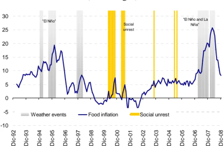
Bolivia has experienced in several times the impact of significant weather events. The largest and most significant of them has been “El Niño” and “La Niña”, characterized by droughts and floods affecting, first crops and livestock, but also deteriorate the roads hindering normal traffic.4 It is remarkable the importance that have taken these environmental phenomena, not only in the magnitude of its impact, but also in the frequency of occurrence. According to INE these increased significantly in recent years (Figure 7).

Figure 7

Natural Disasters in Bolivia by type 2002 - 2007

0 500 1.000 1.500 2.000 2.500 3.000 3.500 4.000 4.500

2002 2003 2004 2005 2006 2007 2008

Inundación Sequía Otros Total

Source: INE.

For example, the manifestation of natural phenomena in 2007 and early 2008 (El Niño in early 2007, frosts in mid-June and La Niña at the end of that year spread to the first quarter of 2008) became one of the most important factors for the rising food prices (Figure 8). Similarly, it is notable the influence of social and political quarrels on inflation.

Figure 8: Food Inflation, weather adverse events and social conflicts 1993 - 2008 (Percentages) -10 -5 0 5 10 15 20 25 30 D ic -9 2 D ic -9 3 D ic -9 4 D ic -9 5 D ic -9 6 D ic -9 7 D ic -9 8 D ic -9 9 D ic -0 0 D ic -0 1 D ic -0 2 D ic -0 3 D ic -0 4 D ic -0 5 D ic -0 6 D ic -0 7 D ic -0 8

Weather events Food inflation Social unrest

"El Niño and La Niña" Social

unrest "El Niño"

Source: BCB based on information from INE.

- Poor Behavior of the Agricultural Sector

The evolution of the agricultural sector measured by the Agricultural Gross Domestic Product (GDP-A) also influenced the price level. Natural phenomena highlighted in the previous section affected in a significant manner agricultural production. Much of 2007, GDP-A recorded negative growth rates that coincided with rising prices for agricultural products and livestock. Just after 2008 the industry began to recover: the reduction of adverse weather effects and the actions implemented by the Government to boost production would have had the expected impact on the sector and also in the behavior of prices (Figure 9).

Figure 9: Food inflation and agricultural production

(Annual change, percentages)

-8 -3 2 7 12 17 22 27 32 Q 1 -9 3 Q 4 -9 3 Q 3 -9 4 Q 2 -9 5 Q 1 -9 6 Q 4 -9 6 Q 3 -9 7 Q 2 -9 8 Q 1 -9 9 Q 4 -9 9 Q 3 -0 0 Q 2 -0 1 Q 1 -0 2 Q 4 -0 2 Q 3 -0 3 Q 2 -0 4 Q 1 -0 5 Q 4 -0 5 Q 3 -0 6 Q 2 -0 7 Q 1 -0 8 Q 4 -0 8

GDP-A (Right Axis) CPI-A (Left Axis)

Source: BCB based on information from INE.

- High Consumption Growth

The relationship between increased consumption and demand for food is important in Bolivia. As mentioned earlier, the average consumption basket of Bolivia shows that about 40% of consumption is spend in food, and this percentage increases when considering a lowest quintile, since in the first two quintiles the food consumption is greater than 50%. Therefore, any increase in the purchasing power of households will lead, to a great extent, in an increased in food demand with the consequent upward pressure on prices at least in the short term, while the supply is adjusting to the increased demand (Figure I.10).

Figure 1.10: Food inflation and private consumption growth

(Percentages) -5 0 5 10 15 20 25 30 35 Q 1 -9 3 Q 4 -9 3 Q 3 -9 4 Q 2 -9 5 Q 1 -9 6 Q 4 -9 6 Q 3 -9 7 Q 2 -9 8 Q 1 -9 9 Q 4 -9 9 Q 3 -0 0 Q 2 -0 1 Q 1 -0 2 Q 4 -0 2 Q 3 -0 3 Q 2 -0 4 Q 1 -0 5 Q 4 -0 5 Q 3 -0 6 Q 2 -0 7 Q 1 -0 8 Q 4 -0 8 -1 2 5 8 CPI-F (Left axis)

Consumption (Right axis)

Source: BCB based on information from INE.

III. Empirical evidence on the transmission of food international inflation to domestic food prices in Bolivia: A VAR Approach5

This section aims to identify the impact of an increase in external food prices on the Bolivian food CPI, through an econometric methodology. In this section, an econometric model (a Vector Autoregressive or VAR) will be estimated to test how long takes the transmission of a non anticipated external food shock and the time of its dissipation.

The database was constructed by taking quarterly series from de Bolivian Central Bank (BCB), INE and the World Bank. Among those: an index of international food prices (

* food t

π _{)6, the total inflation (}πt _{), the domestic food CPI (} food t

π _{), CPI without Food}

( food n t

−

π _{), the total Gross Domestic Product (}yt_{), the Agricultural Gross Domestic Product}

( agri t

y

), Private Consumption ( priv t

C

), the Monetary Base (Mt _{). It should take into account} that in most cases, variables were transformed into logarithms. Also, the series are not stationary in levels, but their first differences are, so they were introduced in the model as

5_{Part of this paper is based on Palmero and Mendieta (2009).}

6

variations. Moreover, the first difference of the log of a series is a good approximation of the growth rate. Annex 1 describes the variables used to estimate this model.

The theoretical model utilizes the McCarthy’s (2006) approach to measure the pass-through from import prices to domestic inflation which uses a VAR. Inflation in period t is assumed to be comprised of several components. One of those is the expected inflation that is form based on the available information at the end of the previous period (t-1). The second, third and forth are the effects of period t “external” shocks, and domestic “supply” and “demand” shocks.

In the particular case of the model of domestic food inflation (π_tfood) we use as proxy of the

external shock the international food inflation (π_tfood*) adjusted by the Bolivian nominal exchange rate. On the other hand and consistent with internal factors described in the previous section, the variables that measure the domestic supply and demand are the rates of growth of Agricultural Gross Domestic Product (ytagri) and Private Consumption (

priv t

C ), respectively.

food t cons t agri t food t food t t food t cons t agri t food t priv t t priv t agri t food t agri t t agri t food t food t t food t c c c E b b C E C a y E y E ε ε ε ε π π ε ε ε ε ε ε π π + + + + = + + + = + + = + = − − − − * 3 * 2 * 1 1 * * 2 * 1 1 * * 1 1 * * 1 * ) ( ) 4 ( ) ( ) 3 ( ) ( ) 2 ( ) ( ) 1 (

The shocks in each equation are the portion of the inflation that cannot be explained using information from period t-1 plus contemporaneous information about domestic external, supply and demand variables. Under these assumptions, domestic food inflation rate are the result of the behavior of the previous inflation and is subject to a series of shocks (internal and external) as is stated in equation (4).

Finally, and following McCarthy op. cit we assume that the conditional expectations (Et−1(•)_{) in each of the above equations can be replaced by linear projections on lags of for}

variables in the system. As quoted by McCarthy “Making this replacement, the model can

be expressed and estimated as a VAR using a Cholesky decomposition to identify the shocks[…] The impulse responses of […] and […] inflation to the orthogonalized shocks of […]provide estimates of the effect of these variables on domestic inflation. In addition, variance decompositions […] enable one to determine the importance of these “external” variables for domestic inflation. In using a Cholesky decomposition to identify the shocks in the model, one issue that arises concerns the identification of aggregate demand and supply

shocks.”

Moreover, following Bhundia (2002), from the Impulse Response Functions (IRF) generated from the VAR model we can build a proxy measure of elasticity as follows:

0 in t ) %( shock after the periods t ) %( t in on

Elasticity * _*

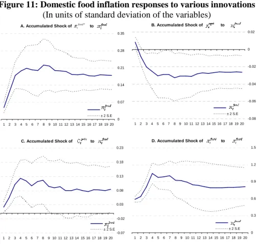
Several shocks are simulated to determine its effects in domestic food inflation. Figure 11 displays in four panels the responses of domestic food inflation of shocks in every variable included in the model.7 The solid line in each panel is the estimated response while the dashed lines denote a two standard error confidence interval band around the estimate. These responses are standardized to correspond to a one percent shock.

Figure 11: Domestic food inflation responses to various innovations (In units of standard deviation of the variables)

A. Accumulated Shock of to

0 0.07 0.14 0.21 0.28 0.35

1 2 3 4 5 6 7 8 9 10 11 12 13 14 15 16 17 18 19 20 ± 2 S.E *

food t

π B. Accumulated Shock of to

-0.08 -0.06 -0.04 -0.02 0 0.02

1 2 3 4 5 6 7 8 9 10 11 12 13 14 15 16 17 18 19 20 ± 2 S.E

C. Accumulated Shock of to

-0.07 -0.02 0.03 0.08 0.13 0.18 0.23

1 2 3 4 5 6 7 8 9 10 11 12 13 14 15 16 17 18 19 20 ± 2 S.E

D. Accumulated Shock of to

0 0.3 0.6 0.9 1.2 1.5

1 2 3 4 5 6 7 8 9 10 11 12 13 14 15 16 17 18 19 20 ± 2 S.E

Source: Own estimates based on a estimated VAR

A shock in international food prices pass-through to domestic-food prices in a couple of quarters. Panel A shows the response of an un-anticipated shock in the international prices and their effect on food inflation in Bolivia. It can be seen that the increase is transmitted on a contemporary way, reaching its maximum impact after four quarters, then beginning to stabilize.

An increase in Agricultural GDP reduces internal food prices. With regard to the effect of an un-anticipated shock in theytagri, panel B shows how this shock, equivalent to an

7 _{The reduced form residuals from the VAR are orthogonalized using a Cholesky decomposition to identify the}

structural external an internal shocks.The number of lags was chosen under the Akaike and Schwartz criteria that

reported the inclusion of 4 lags in each model. This number allows capturing the entire dynamic of the series and eliminates the problems of autocorrelation and heteroscedasticity. In the same line, the roots of the characteristic

increase in agricultural production translates in a sharp decline in inflation in the first three quarters and reaches its maximum effect after and a half with permanent effects on prices. A demand shock (measured as an increase in consumption) put pressure on food prices. The effect of increasing levels of private consumption on food prices, while keeping everything else constant, drives the price level to a maximum after three quarters and then corrected downwards from the fourth until the sixth quarter, time from which the effect begins to decline and stabilizes after approximately three years. Panel C shows that the increase in consumption generates permanent effects on price levels.

Movements in international food prices explain more than 20% of the error in forecasting. Variance decomposition analysis shows the percentage of variance of the error in forecasting several periods ahead that is explained by each of the variables of the system. From Table 1 it can be inferred that after three quarters 23% of the forecast error is explained by external food inflation, 12% for the evolution of agricultural GDP, 5% by growth consumption and 59% by the domestic food inflation itself. After 20 quarters (5 years), the results are relatively similar recording slight decreases in both external and internal food inflation, a significant increase in consumption, while the ytagri remains almost unchanged.

Table 1: Decomposition of variance of the CPI-F

Período

1 7.51 6.16 1.29 85.04

2 17.24 11.69 2.19 68.89

3 23.10 12.10 5.04 59.76

4 21.02 11.10 5.23 62.65

5 20.83 11.57 5.51 62.09

10 21.25 11.23 7.30 60.22

15 21.19 11.36 7.64 59.81

20 21.23 11.35 7.78 59.63

* food t

π

Source: Own estimates based on a estimated VAR

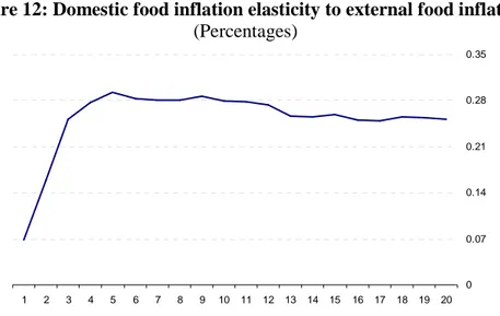
Figure 12: Domestic food inflation elasticity to external food inflation (Percentages)

0 0.07 0.14 0.21 0.28 0.35

1 2 3 4 5 6 7 8 9 10 11 12 13 14 15 16 17 18 19 20

Source: Own estimates based on a estimated VAR

IV. Effect of international food inflation in the context of a Small Structural Macroeconometric Model (SSMM)

For a better understanding of the effects of international food inflation in the economy (not only in inflation), it was used a SSMM. The main benefits of the use of this model are: i) it is a general equilibrium framework which incorporates besides inflation, economic activity, monetary (and sometimes fiscal) policy, exchange rate behavior, among others; ii) it includes expectations about the future evolution of the main variables; and, iii) their relationships can be derived from microeconomic foundations. More details about these models are shown in Annex 1.

The SSMM was modified to include main characteristic of Bolivian economy. In the particular case of the Bolivian economy, Mendieta, Palmero and Murillo (2008) estimated an SSMM, which differs from the conventional structure, due to two factors: the inclusion of an exchange rate rule consistent with the exchange rate regime (crawling peg) and the exclusion of an interest rate rule, because the BCB has focused in monetary aggregates and the credit channel has been limited. More details about this SSMM (equation specifications, estimates and limitations) are in Annex 2.

The main feature of this SSMM is the use of an exchange rate rule instead of nominal interest rate, consistent with the degree of dollarization of the Bolivian economy. The rule for determining the nominal exchange rate depends on the gap between the observed and inflation target8, the real exchange rate misalignment (in levels and growth rates) and the output gap. Besides, this relationship exhibits high inertia due to the high degree of dollarization, especially in the financial system. Dollarization is related to the cost of

8 _{Although BCB has not adopted a Full-Fledged Inflation Targeting Regime, since 1995 it announces a target}

moving exchange rate; and it explains the high inertia in exchange rate rule as is expected by theory of economic policy with adjustment costs (Turnovsky, 1977).

This feature has some earlier empirical evidence. The estimation of a exchange rate rule has three main precedent studies: one specifically applied to Bolivia (Parrado, Maino and Leiderman, 2006), one applied to Singapore (Parrado, 2004) and one applied to Central America countries (Jacome and Parrado, 2007). It is convenient to point out that in most of central banks, monetary policy decisions do not use specifically a strict rule; but, central bankers act as if they have one in mind.

The exchange rate has an important role in the economy. This is given through two ways: its effect in the interest rate (a weighted rate of US and local credits, expressed in Bolivianos) and the real exchange rate misalignment. Both imply a negative relationship between exchange rate and output gap, specially the first one. It is rationalized by an income effect and “balance sheet” effects. Then abrupt movements in exchange rate could have perverse effects in the economy. This fact explains that, according Parrado, Maino and Leiderman op.cit., Bolivia followed a “Fear of floating competitiveness targeting” scheme, where the primary target is competitiveness and the secondary one is inflation; the operational target is the rate of crawl; and the primary shock absorber is foreign assets and the secondary one is the interest rate. As it is shown in Annex 2.2., the estimated rule shows more evidence in the same way.

The SSMM can capture the effect of movements in international food prices. To analyze the transmission of international food inflation has been added an equation relating this variable with non-core inflation though Bolivian food inflation. Besides, there is an indirect effect through external inflation relevant for Bolivia. Figure 13 describes these ideas:

Figure 1.13: Transmission mechanism of monetary policy in the case of Bolivia

International food inflation

Non Core Inflation

External inflation Core Inflation

Total CPI inflation

Indirect channel Direct channel Bolivian food

inflation

International food inflation

Non Core Inflation

External inflation Core Inflation

Total CPI inflation

Indirect channel Direct channel Bolivian food

inflation

increase in external inflation and higher inflation would lead to a reduction of real interest rate (Figure 14).

Figure 1.14: Impulse response analysis to a rise in international food inflation

Source: Own estimates based on a modified SSMM

Note: oya = over year ago

Figure 15: Simulation of the effect of 2006Q4-2008Q2 international food inflation on Bolivia total inflation

0% 2% 4% 6% 8% 10% 12% 14% 16% 18% 2 0 0 6 Q 1 2 0 0 6 Q 2 2 0 0 6 Q 3 2 0 0 6 Q 4 2 0 0 7 Q 1 2 0 0 7 Q 2 2 0 0 7 Q 3 2 0 0 7 Q 4 2 0 0 8 Q 1 2 0 0 8 Q 2 2 0 0 8 Q 3 2 0 0 8 Q 4 2 0 0 9 Q 1 Total inflation

Inflation less food prices shock

Source: INE and own estimates

V. Concluding Remarks

Based on the results obtained in this chapter, the following conclusions and final thoughts are extracted.

Bolivian food and headline inflation is determined by internal and external factors. External food prices, the behavior of agricultural GDP, climatic conditions and the dynamics of private consumption are the main factors that determine the evolution of Bolivian food inflation, and then, headline inflation.

External food inflation is one of the main drivers of Bolivian food inflation. Global food prices have a significant impact that is transmitted with lags and have a permanent effect on domestic price level. An important part of the articles included in the CPI (food and headline) are tradable. So that, changes in prices of these goods affects directly and indirectly to local prices. The direct channel is derived from imported consumer goods, while the indirect effects are originated by imported capital goods and raw materials, essential for internal production of final goods.

Econometric evidence shows that the pass-through from external to domestic food inflation is relevant. A structural VAR estimated for Bolivian economy shows that the factors mentioned above are important in the evolution of domestic food inflation. Specifically, an unanticipated shock in global food prices drives an increase of 25% in domestic food inflation in the long run.

of this shock must be analyzed in the context of a general equilibrium model, which have to include the main characteristics of the economy and the policy responses. In this way, a SSMM was estimated, which primarily includes a relationship to determine core and headline CPI (a New-Keynesian Phillips curve), another for the determination of output gap (an IS curve) and a policy rule (in the case of Bolivian economy, an exchange rate rule). It was modified to include international and domestic food prices.

References

Agénor, P. (2004). The Economics of Adjustment and Growth 2nd. Ed., Cambridge, Harvard University Press.

Berg A., Karam P., and Laxton D. (2006), “A Practical Model-Based Approach to

Monetary Policy Analysis—Overview”, International Monetary Fund, Working Paper

WP/06/80.

Berg A., Karam P., and Laxton D. (2006a), “A Practical Model-Based Approach to

Monetary Policy Analysis - A How-To Guide”, International Monetary Fund,

Working Paper WP/06/81.

Bhundia A. (2002), “An Empirical Investigation of Exchange Rate Pass-Through in South

Africa”. IMF’s Working Paper No. 165, International Monetary Fund, Washington.

Calvo, G. (1979) “Staggered Prices in a Utility-Maximizing Framework” Journal of

Monetary Economics 12 (3), Sept.:983-998.

Central Bank of Bolivia (2009). Monetary Policy Report January 2009. Available on the website http://www.bcb.gov.bo/

Central Bank of Bolivia. Economic Statistics available on the website

http://www.bcb.gov.bo/

Clarida, R; J. Gali and M. Gertler (1999) “The Science of Monetary Policy: A New Keynesian Perspective” Journal of Economic Perspectives 37 (4): 1661-1707.

Cossío J. Laguna M., Martin D., Mendieta P. Mendoza R., Palmero M. and Rodriguez H. (2008), “Inflation and Central Bank Policy in Bolivia”. Central Bank of Bolivia, Analysis Review Edition 10th – 2008.

D’Amato L., Garegnani L. (2006), “The dynamics of inflation in the short term: the

estimation of a neo-keynesian hybrid Phillips curve for Argentina”. Monetaria,

Vol.XXIX (4), October - December.

Easterly W. (2006): “An Identity Crisis? Examining IMF Financial Programming”. World

Development, Vol. 34, No. 6, June.

Economic Commission for Latin America and the Caribbean (2008) "Preliminary Overview of the Latin America and the Caribbean Economies " United Nations. Edwards S. (1989): “The International Monetary Fund and the Developing Countries: A

Critical Evaluation”. Carnegie-Rochester Conference Series on Public Policy, 31:7-68 (The Netherlands: Elsevier Science Publishers, North-Holland).

Favero C. (2001) Applied Macroeconometrics. London, Oxford University Press.

Habermeier K., Ötker-Robe I., Jacome L., Giustiniani A, Ishi K., Vávra D., Kışınbay T., and Vazquez F. (2009) “Inflation Pressures and Monetary Policy Options in

Emerging and Developing Countries: A Cross Regional Perspectiva” Working Paper

WP/09/1, FMI.

International Monetary Fund (2009) “Bolivia: 2008 Article IV Consultation—Staff Report;

Statement by the Executive Director for Bolivia” Country Report No. 09/27 January 2009.

Jacome, L. and E. Parrado (2007). "The Quest for Price Stability in Central America and the Dominican Republic," IMF Working Papers 07/54, International Monetary Fund Lucas, R.E. Jr (1976), “Econometric Policy Evaluation: A Critique”, en K. Brunner y A.

Meltzer (Eds.). The Phillips Curve and Labor Markets. Amsterdam: North-Holland, Luque J. y M. Vega (2004) “Usando un Modelo Semi-Estructural de Pequeña Escala para

hacer Proyecciones: Algunas Consideraciones” Estudios Económicos No. 10, Banco Central de Reserva del Perú.

Mendieta, P. and H. Rodriguez (2008) “Price’s formation and monetary rules in a

dollarized economy”, Unpublished document.

Mendieta, P. and Rodríguez H. (2007), “Featuring a neo-keynesian Phillips curve for a

highly dollarized economy: The case of Bolivia”. Paper presented at the First Latin

American Seminar on Economic Models and Projections in Central Banks, held in Buenos Aires, April 26th.

Mendieta, P.; M. Palmero and A. Murillo. (2008), “Estimation of a Small Structural Model

for Bolivia”, Central Bank of Bolivia Working Paper Nº 2.

National Institute of Statistics. Economic Statistics available on the website

http://www.ine.gov.bo/

Palmero, M. and P. Mendieta (2009) “The effect of international prices on Bolivian prices” Paper presented at the Center for Latin American Monetary Studies (CEMLA in spanish).

Parrado E. (2004) “Singapore’s Unique Monetary Policy: How Does It Work?” IMF Working Paper WP/04/10, International Monetary Fund.

Parrado, E.; R. Maino and L. Leiderman (2006). "Inflation Targeting in Dollarized Economies," IMF Working Papers 06/157, International Monetary Fund.

Pesaran, M.H., and Y. Shin, (1998), “Generalized Impulse Response Analysis in Linear

Multivariate Models”, Economics Letters, Vol.58, pp.17-29.

Polak, J. J. (1957): “Monetary analysis of income formation and payments problems”. IMF

Staff Papers 6.

Robichek, E. W. (1971): “Financial Programming: Stand-By Arrangements and Stabilization Programs”, IMF, January.

Robichek, E. W., “Financial Programming Exercises of the International Monetary Fund in Latin America”. Mimeo, Rio de Janeiro, 1967.

Rodriguez H. (2007), “Potential Output”, Paper presented at the Latin American Seminar on Joint Research on Non-Observable Variables performed in Buenos Aires, April 27th 2007.

Rotemberg, J. (1984) “A Monetary Equilibrium Model with Transaction Costs” Journal of

Turnovsky, S. (1977). Macroeconomic Analysis and Stabilization Policy. Cambridge, Cambridge University Press.

Vega, M. (2007) “El Modelo de Proyección Trimestral (MPT)” Document of the Macroecomic Models Department at Banco Central de Reserva del Perú.

World Bank. Commodity Prices Index Database from Global Economic Monitor. Available

on subscription via the online website

Annex 1:

Description of Variables Used in VAR model

Variable Acronym Description Source

External Food Price Index CPI-F* Prices index of the main food products traded in international markets.

Global Economic Monitor - World Bank Consumer Price Index CPI Base 1991 to March 2008 and Base 2007 hereafter INE Domestic Food Price Index CPI-F Calculated by CBB based on CPI data INE Price Index without Food and Beverages CPI-WF Calculated by CBB based on CPI data INE

External Price Index EPI

Inflation measures the change in its external relevance to Bolivia. Inflation is calculated as the trading partner countries weighted by their weight in foreign trade, expressed in dollars.

CBB

External Gross Domestic Product GDP-E Corresponds to the external growth relevant to

Bolivia calculated the same way that the EPI. CBB

Agricultural Gross Domestic Product GDP-A Gross domestic product at constant prices by

economic activity: agriculture, sylviculture, hunting and fishing. INE Gross Domestic Product GDP Gross domestic product at constant prices. INE Private Consumption PC Gross domestic product by type of spending: private consumption. INE Monetary Base MB Measure of money that is the primary basis of the monetary

aggregates. CBB

Real Exchage Rate RER Calculated based on the 17 main trading partners of Bolivia. CBB Purchasing Exchange Rate PER Determined on a daily basis by the CBB's Bolsín. CBB Bolivianization Bol Variable that measures the financial remonetization process. CBB

Government Spending GS Gross domestic product by type of spending: consumption spending in the public sector.

INE- Ministry of Economy and Public

Finances Dummy Variable 1 Dum1 Captures the effects of adverse weather and some social unrest

Annex 2:

SSMM in the context of economic modeling and its main characteristics

Monetary policy generally affects the economy with lags and there are different transmission mechanisms (credit channel, expectations, exchange rate, among other) and they are specific for each country. For this reason, central banks have emphasized the use of economic and econometric models that can replicate the main empiric regularities of the economic cycle to take the pertinent actions.

Previous to the eighties, this interest was focused in the estimation of econometric models including many static relationships or with a very simple dynamic structure for an important group of variables (Favero, 2001). However, these models failed in policy analysis and forecasting.

Alternatively, accounting models were used, like Financial Programming, based primarily in the monetary approach to the balance of payments (Polak, 1957 and Robichek, 1967 and 1971) and static models based on this initial approach as 1-2-3 or RMSX models, among others (Agenor, 2004). However, their use has been questioned too (Edwards, 1989 and Easterly, 2004), since they only guarantee accounting consistency and main relationships, as the stability of the velocity of money, the effective control of liquidity by central banks, among others, seem implausible empirically.

In contrast, econometric models improved gradually their capacity to replicate dynamic characteristics of economic series, with the use of new techniques, especially the estimation of co-integration models (long run relationships) and error correction models (short run relationships but consistent with long run ones). Nevertheless, the critic to conventional econometrics from the Prize Nobel Robert Lucas in 1976 pointed out the limitations of the use of these tools for macroeconomic analysis. In synthesis, Lucas argued that changes in economic policy affect the estimated parameters of equations, invalidating forecasting and even the analysis.

Then, econometric relationships without economic structure, as VAR were more popular among central banks, since they were able to replicate the dynamics of economic variables and they were not based in particular theories. However, the last one was its main weakness.

Due to these theoretical and empiric limitations, the development of new models called Real Business Cycles (RBC) was a landmark for economic modeling, because they tried to combine micro-economic foundations of macroeconomics with the dynamic properties of variables. From them, Dynamic Stochastic General Equilibrium (DSGE) models were developed, which consist in tools consistent with conventional economic theory, but with the capacity to replicate empirical regularities of the economic cycle. For this reason, they are immune to previously mentioned Lucas's Critique.

A special cases of these models are the Small Structural Macro-econometric Models (Berg, Karam and Laxton, 2006a and 2006b), because they use a basic structure to construct a general equilibrium model. They are broadly used across the world, including developing countries. In its basic form, they include:

the output gap through the labor supply equation.9 Another assumption to include lagged inflation goes in line with Clarida, Gali and Gertler (1999), to form an hybrid version (forward and backward looking behavior):

(

)

1 1 1 1 1 2 1

c

t t Et t yt t

π

π =α π− + −α π+ +α − +ε

• The evolution of output gap is described by a new IS curve. Its microeconomic foundation is obtained from the dynamic optimization of consumption (the log-linearized version of the Euler equation, that relates actual and future consumption with the behavior of real interest rate) and an investment function (usually with adjustment costs, also related to interest rate). In formal terms, it relates actual output gap (y) with expected and lagged gap, real interest rate (R) gap and real exchange rate (z) miss-alignment:10

* *

1 1 2 1 3( 1 1) 4( 1 1)

y

t t t t t t t t t

y =β E y₊ +β y₋ +β R₋ −R₋ +β z₋ −z₋ +ε

• A monetary policy rule (called Taylor rule), which describes the response of the authority against deviations from the target variables (usually inflation and output). Svensson (1997) and further studies show that it can be derived from a minimization of a central bank loss function, given the previous two equations.

(

)

1 2 3

i

t t t t t t t

i = + = +R π γ γ π π− +γ y +ε

• In the case of open economies, Uncovered Interest Parity (UIP) for the determination of exchange rate is added, which can be adjusted for risk premium.

As Table A1.1 shows, they are used in many central banks and international organizations for economic analysis and forecasting purposes.

Table A1.1: Use of SSMM and DSGE in selected countries or regions

Country SSMM DSGE Country SSMM DSGE

Argentina U D (ARGEM) Italy U D

Australia U Japan U

Belgium U Namibia U

Bolivia U (MEP) D New Zealand U (QPM)

Canada U (QPM) D (TOTEM) Norway D (NEMO)

Chile U (MEP) MAS Peru U (MPT)

Colombia U D (PATACON) South Africa U

Czech Republic U (QPM) D Sweden U

European Union U D Switzerland U D

IMF U U (GEM) U.S.A. U (FRBUS) SIGMA

Israel U United Kingdom U U

Source: Adapted from Vega (2007)

Notes: U=Used by CB. D=Developing. Between brackets are the models’ names.

9 _{This analysis could be refined using a proxy of marginal cost and it is in the BCB further research agenda.} 10 _{The gap of variable x is the difference or log-difference between actual and potential (steady-states) values.}

Annex 3:

The SSMM estimated for Bolivian Economy

The SSMM was modified to take into account main particularities of the Bolivian Economy. The SSMM estimated has 3 of 4 equations included in a standard model, one of them modified: A New Keynesian Hybrid Phillips Curve for the core inflation, an IS equation modified to include competitiveness, external output and fiscal expenditure and a policy rule for the exchange rate. Then, it does not include a monetary policy rule for the interest rate and the Uncovered Interest Parity for the exchange rate. Table A3.1, at the end of this section, explains the definitions and notation employed below.

The Phillips curve captures the dynamic of core inflation, including expectations. This equation comes from a variation of estimates of Mendieta and Rodriguez (2007 and 2008), whom rationalizing the approach of D'Amato and Garegnani (2006) for Argentina, indicating that at the time of forming a price, one part of the firms instead of just taking the past information, they use a set of information, which in this case also includes foreign inflation and exchange rate movements. The equation has been used to model core inflation:

(

)

t t t

t c

t t c

t c

t E y e

π ε π α α

α π α π

α

π = 1 −1+ 1− 1 +1+ 2 −1+ 3∆ −1+ 4 *−1+

A priori it is expected that all parameters will be positive. Furthermore, although not restricted in the estimation, it implies that inflation is a weighted average of the public expectations plus the own inflation inertia. In economies where the central bank has more credibility, it is expected that α1 to be large. More advanced models assume that instead of a relationship with the gap, there is a relationship with the marginal costs. Unfortunately, in the case of Bolivia, it is impossible to construct this variable because of the low regularity of labor statistics.

Consistent with studies on the Phillips curve, the most direct channel to affect inflation is the exchange rate. The indirect channel, which is more usual in other economies, occurs through the output gap, which is affected by the interest rate, the main instrument of macroeconomic policy in other countries.

The output gap is related to other four gaps: interest rate, real exchange rate, external output and fiscal expenditures. The IS equation is:

(

)

t t t t

t t

t t

t t

t t

t E y y R R z z yext yext g g

y =β_{1 +1}+β_{2 −1}+β₃( ₋₁− *₋₁)+β₄( ₋₁− *₋₁)+β₅( − *)+β₆ − * +ε

It is expected that the parameters would have a positive sign, except for β3. In the last case, according to the theory, an increase of interest rate would discourage demand by its contractionary effect on consumption and investment. Because of low financial market development, particularly investment might be expected that β3 is small in absolute terms

Although in most cases it is expected that the effect of real depreciation is positive, for its effects on exports, for dollarized economies like Bolivia could be negative because of the effects on real incomes (if it is assumed transactions’ dollarization) and the effect on the balance sheet of firms and financial institutions, was constructed in such a way that an increase shows a depreciation and a fall a currency appreciation.

The rule of monetary policy is an exchange rate rule. One of the key roles of monetary policy is to provide the public with a nominal anchor that allows identifying the stance of monetary policy (contractionary or expansionary). The monetary rule is the variable that fulfills this role. Usually, the central bank determines monetary policy by using some kind of interest rate on short-term, or, each time less, through monetary aggregates. However, as was demonstrated by Parrado (2004 and 2006) for Singapore and Bolivia, the conduct of monetary policy can be performed by an exchange rate rule.11

Although Bolivia does not have an anchor inflation formally defined, the monetary policy stance has been based on the position regarding the movement of the nominal exchange rate, based on a crawling peg regime that consists of un-announced and gradual movement of parity. Under these assumptions and in the direction of Mendieta and Rodriguez (2008), the rule for the nominal exchange rate is:

e t t t t t t t t t

t e y z z

e = + ∆ ₋ + ₋ + ₋ − ₋ + − + − + ∆

∆

δ

δ

δ

δ

π

π

δ

π

π

δ

ε

It is expected that all coefficients will be negative, except δ_4.

These main equations were estimated with a method to avoid endogeneity bias and use actual variables to approximate expected ones. Equations were estimated with the Generalized Method of Moments (GMM). Next, they were calibrated in suitable programs designed for this task.12 Results are shown in Table A3.2, below this Annex.

To include the effect of international food inflation were added other equations. International food inflation has effects in two ways: i) Expressed in local currency, it is a determinant of Bolivian food inflation, which is related to non-core inflation; and ii) It affects external inflation, and by this way, core inflation. In formal terms:

( )

( )

(

( )

)

In the case of Singapore the motivation is different, since the country uses the exchange rate because of its high capital mobility environment where the interest rates are similar to international ones.

12

Where A(L) and B(L) are polynomials of the lag operator (L).13 Because there are not endogeneity problems these equations were estimated with the usual Ordinary Least Squares (OLS) technique.

Mostly, the results of estimation were consistent with the expected signs and magnitudes. They are shown in Table A2.2. The main difference with standard results is the contractionary effect of a real depreciation, but explained by the high degree of dollarization of the Bolivian economy.

This SSMM has some limitations to be taken into account. The first is the scope of the data used, especially in the measurement of economic activity, because Bolivia has a large informal sector. However, the GDP reported by INE is the unique proxy for this variable and the estimates of equations that include this series seems plausible. An additional argument comes from the Central Bank of Peru, a country with wide informal sector as Bolivia, which has used this model successfully in the last years to analyze and forecast inflation (Luque and Vega, 2003). Colombia is other useful example.

13

Table A3.1: Definition of main variables used in the SSMM

Variable Definition Observations

c t c t c t p p 1 − ∆ =

π Core inflation

Quarterly percentage change of Core CPI (p_tc), which is defined as total CPI less perishable food and regulated prices.

     

=log _*

t SA t t PIB PIB y Output gap

Log-difference between the seasonal adjusted GDP not including mining and hydrocarbons ( SA

t

PIB ) and

potential GDP ( * t

PIB ). The last one was obtained

using a Hodrick – Prescott (HP) filter with a factor specific for Bolivia (λ=7185), according Rodriguez (2007).

t

e Nominal exchange

rate

Official exchange rate fixed by the BCB in daily auctions in the Bolsín (sell exchange rate).

* t

π External inflation in U.S. dollars

Quarterly percentage change of an index of Bolivia’s 13 main partner countries inflation, expressed in U.S. dollars.

t

R Real interest rate

It corresponds to (Rt = it – πt). 14

Furthermore, to include financial dollarization, the nominal interest rate is a weighted average of rates on domestic and foreign currency expressed in domestic currency.15

* t

R denotes the natural interest rate, estimated in a similar way as the potential output. Therefore, the difference measures the gap between the real interest rate with respect to its natural or potential level.

t

z Real exchange rate

Correspond to the multilateral real exchange rate index calculated by the BCB, taking into account the main trade partners of Bolivia. Then, z_t−z*_t is the exchange rate misalignment.

t

yext

External output relevant for Bolivian economy

It is measured as an average of the GDP of the most of the 13 major trading partners of the country, weighted by their share in foreign trade. With an asterisk denotes the potential external output.

t

g Growth of fiscal

expenditures

It measures the quarterly growth of seasonally adjusted expenditures of central government. With an asterisk denotes the trend growth.

nc t

π Non-core inflation Quarterly percentage change of Non Core CPI (perishable food and regulated prices).

14

Unlike other models that use the expression R_t =i_t −E_tπ_t+1, in the case of Bolivia the rate of inflation is directly used, because according to the results of the Economic Expectations Survey of the BCB was noted that expected inflation has co-movements respect to the observed one.

15

This variable is the average weighted active interest rate of banking system, according to the following formula: $ 1 / 1 ˆ 1 us

Bol Dol Dol t

t t t t t t

t

i

i Bol i Dol i i

e

+

= × + × = −

+

Table A3.1: Definition of main variables used in the SSMM (Cont.)

Variable Definition Observations

t

π Total inflation

Is defined as χπ_tc+

(

)

Bfi t

π Bolivian food

inflation

Quarterly percentage change of Bolivian food CPI (p_tBfi), which includes food and beverages.

Wfi t

π International food inflation

Quarterly percentage change of international food prices index, calculated by The World Bank.

Oil t

Table A3.2: Estimation Results of a SSMM for Bolivia

i) Phillips Curve:

(

)

t t t t c t t c t c

t E y e

π ε π α α α π α π α

π = 1 −1+ 1− 1 +1+ 2 −1+ 3∆ −1+ 4 *−1+

1 α 0.578 (0.048) 2 α 0.242 (0.078) 3 α 0.193 (0.046) 4 α 0.068 (0.031)

ii) IS Curve:

(

)

t t t t t t t t t t t t

t Ey y R R z z yext yext g g

y =β ₊ +β ₋ +β ₋ − ₋ +β ₋ − ₋ +β − +β − * +ε

6 * 5 * 1 1 4 * 1 1 3 1 2 1

1 ( ) ( ) ( )

1 β 0.617 (0.086) 2 β 0.180 (0.047) 3 β -0.033 (0.020) 4 β -0.045 (0.014) 5 β 0.214 (0.075) 6 β 0.050 (0.010)

iii) Exchange rate rule:

e t t t t t t t t t

t e y z z

e = + ∆ ₋ + ₋ + ₋ − ₋ + − + − + ∆

∆ δ₀ δ_{1 1} δ_{2 1} δ₃(π ₁ π ₁) δ₄(π π*) δ₅( *) ε

1 δ 0.740 (0.023) 2 δ -0.051 (0.013) 3 δ -0.023 (0.008) 4 δ 0.006 (0.001) 5 δ -0.051 (0.004)

iv) Non core inflation:

( )

t Bfi t nc t nc

t AL

π ε π κ π κ

π = 0+ −1+ 1 +

1

κ S.R.: 0.197 L.R.: 0.459

(0.022)

iv) Bolivian food inflation:

( )

(

( )

)

t Wfi t t Bfi t Bfi

t B L e

π ε π µ π µ

π = ₀+ ₋₁+ ₁ ∆ln + +

1

µ S.R.: 0.124 L.R.: 0.574

Table A3.2: Estimation Results of a SSMM for Bolivia (Cont.)

iv) External inflation in U.S. dollars:

*

3 2

* 1 1 0

* ζ ζ π ζ π ζ π επ

π t

Oil t Wfi t t

t = + − + + +

2

ζ S.R.: 0.155 L.R.: 0.194

(0.082)

3

ζ S.R.: 0.075 L.R.: 0.093