Complexity of XOR/XNOR Boolean Functions: A Model using Binary
Decision Diagrams and Back Propagation Neural Networks
Ali Assi
Department of Electrical Engineering, United Arab Emirates University, UAE
P.W.C. Prasad and Azam Beg
College of Information Technology, United Arab Emirates University, UAE
V.C. Prasad
Faculty of Engineering, Multimedia University, Malaysia
[email protected]
ABSTRACT
This paper proposes a model that predicts the complexity of Boolean functions with only XOR/XNOR min-terms using back propagation neural networks (BPNNs) applied to Binary Decision Diagrams (BDDs). The BPNN model (BPNNM) is developed through the training process of experimental data already obtained for XOR/XNOR-based Boolean functions. The outcome of this model is a unique matrix for the complexity estimation over a set of BDDs derived from Boolean expressions with a given number of variables and XOR/XNOR min-terms. The comparison results of the experimental and BPNNM underline the efficiency of this approach, which is capable of providing some useful clues about the complexity of the circuit to be implemented. It also proves the computational capabilities of NNs in providing reliable classification of the complexity of Boolean functions.
Key words: Binary Decision Diagrams (BDDs), Reduced Ordered Binary Decision diagrams (ROBDDs), XOR/XNOR min-terms, Complexity, Boolean Functions.
1. INTRODUCTION
The continuous increase of integration level of modern digital circuits imposes high and increasing needs for methods and algorithms used in VLSICAD design verification and testing [1], [2], [3]. The efficiency of any method depends on the complexity of Boolean functions representing circuits under test and verification. Research on the complexity of Boolean functions using non-uniform computation models is today an active research area in theoretical computer science [4], [5]. It has a direct relevance to practical problems in the CAD of digital circuits.
ROBDD is an efficient structure for representing and manipulating Boolean functions symbolically and has been successfully applied to solving many problems in VLSICAD [4], [5], [6]. The BDD representation is defined and proposed by Akers [7] and extended by Bryant [8]. BDDs are compact representations for many functions and lend themselves for fast execution of logical operations. One of the constraints required to achieve canonicity is the ordering imposed by the input variables [9]. The size of ROBDD, measured in number of nodes it contains, depends on this order and may vary drastically from one ordering method to the other. Some functions, such as adders, lead to a BDD size that exponentially or linearly varies with the number of variables depending on the variable order selection [9]. Due to memory and processing-time constraints associated with real world CAD applications, it is important to minimize the ROBDD size as much as possible [10], [11].
BPNNs are common classes of artificial NNs. They are named after a very familiar teaching method for NNs
called the Back-Propagation. Some examples of inputs and their corresponding known-correct outputs are presented to the BPNN. Internal structures of the BPNN are then numerically adjusted to iteratively improve the difference between the input and desired outputs [12], [13], [14]. A lot of research works have been carried out to study the relationship of Boolean function and NN [15] as well as to analyze the measure of the Boolean function complexity related to their implementation in NN [15].
The base of this work is the mathematical model obtained for the BDD complexity using XOR/XNOR min-terms [16]. In this work we apply the BBNN method to ROBDD to estimate the complexity of Boolean function with only XOR/XNOR min-terms. The proposed BPNNM provides good alternative to other methods previously proposed by the same authors. In section 2 we provide some background information pertaining to BDDs and NNs. Section 3 reviews the previous works done by the same authors on the estimation of BDD complexity based on mathematical models. The proposed BPNNM for the complexity estimation of Boolean functions with only XOR/XNOR min-terms is explained in the 4th and 5th sections. Finally we conclude this paper with our future developments.
2. PRELIMINARIES
2.1 Binary Decision Diagram (BDD)
Basic definitions for binary decision diagrams are detailed in [6], [7], [8], [9].
Definition 1:A BDD is a directed acyclic graph (DAG). The graph has two sink nodes labeled 0 and 1, representing the Boolean functions 0 and 1. Each non-sink node is labeled with a Boolean variable v, and has two out-edges labeled 1 (or then) and 0 (or else). Each non-sink node represents the Boolean function corresponding to its 1 edge if v=1, or the Boolean function corresponding to its 0 edge if v=0.
Definition 2: An Ordered Binary Decision Diagram
(OBDD) is a BDD in which each variable is encountered no more than once in any path and always in the same order along each path.
Definition 3: A Reduced Ordered Binary Decision
Diagram (ROBDD) is an OBDD where each node
represents a distinct logic function. It has the following two properties:
(ii) If two nodes point to two identical sub-graphs (i.e. isomorphic sub-graphs), then one sub−graph will be removed and the remaining one will be shared by the two nodes.
2.2 Neural Networks (NNs)
[image:2.595.315.498.70.194.2]NN mimic the ability of a human brain to find patterns and uncover hidden relationships in data. NNs can be more effective than statistical techniques for organizing data and predicting results, and are very efficient in modeling non-linear systems [17], [18], [19]. A NN is defined as a computational system comprising of simple but highly interconnected processing elements (PEs) ( or neurons) ( Figure 1) [13]. PEs are NN equivalents of biological neurons. Similarly, neural network interconnections are equivalents of synapses that connect a neuron to others. Information is processed by the PE’s by dynamically responding to their inputs. Unlike conventional computers that process instruction and data stored in the memory in a sequential manner, the NNs produce outputs based on a weighted sum of all inputs in a parallel fashion.
Figure 1. Processing element (PE) – building block of a neural network
In Figure 1 the inputs (i(0)..i(n-1)) to a PE are scaled with weights (w(0) .. w(n-1)) and summed up before being passed through an activation function. The activation function determines whether a PE activates (fires) or not. A sigmoid (non-linear) activation function has an s-shaped output between the limits [0, 1]. The function (1) is defined as [20]:
)
1
(
1
x
e
Y
−+
=
(1)Each input of an NN corresponds to a single attribute of the system being modeled. The output of the NN is the prediction we are trying to make. Figure 2 shows the topology of a simple 5-layer feed-forward NN with 2 inputs and one output.
The NN has 2 input neurons (PE(ip1), PE(ip2)), three hidden layers with 5 neurons each (PE(hnm) is the mth neuron in nth hidden layer), and one neuron in the output layer (PE(op1)) [20]. The BPNN is fully-connected, meaning; all neurons in one layer connect to all neurons in the next layer. NNs use different types of learning (or training) mechanisms, the most common of them being supervised learning. In this method of learning, a set of inputs is provided to the NN and its output is compared with the desired output.
Figure 2. Topology of 5-layer feed-forward neural network
The difference between the actual and the desired outputs is used to adjust the weights (Figure 1) to different PEs in the network. The process of adjusting weights is repeated until the output falls within an acceptable range.
To ensure a robust NN design, the set of input data and corresponding output data has to be chosen carefully. The input-output data set for an NN is called a training set. Additionally, special attention has to be paid to the formatting and scaling of the data for effective NN training [20]. The available data is divided into training and validation sets. An NN is only trained with the training set. Validation set is run on the NN to verify that the inputs are producing desirable outputs. If the validation phase produces large deviations, the training set or the network structure needs to be examined; re-training is required in this case [20].
3. PREVIOUS WORK
In this section we briefly describe the background concept and results achieved in the area of the estimation of BDD complexity prior to introducing the BPNNM.
3.1 Relation between the Size of a Boolean function and the BDD Complexity
The complexity of the ROBDD mainly depends on the number of nodes represented by the BDD. An experiment was done in [21] to analyze the complexity variation in BDDs i.e. the relation between the number of product terms and the number of nodes for any number of variables. The experimental and equation graph (Figure 3) shows that the complexity of the BDD can be modeled mathematically by (2).
1 )
( +
⋅ ⋅
=
α
β −NPT⋅γ e NPTNN (2)
where, NN is the number of nodes that represents the complexity of the BDD, NPT is the number of non-repeating product terms in the Boolean function,
α
,β
andγ
are three constants. Using curve fitting techniques, the variations of α, β and γ were mathematically modeled and represented by the following equations (3), (4) and (5).) 51 . 1 063 . 0 ( 9855 .
0 ⋅e ⋅NV
=
α
(3)) 298 . 1 ( )
01552 . 0 (
2072
.
67
03115
.
1
⋅
e
− ⋅NV+
⋅
e
− ⋅NV=
β
(4)) 5072 . 1 ( )
4188 . 0 (
9723
.
41
96228
.
0
⋅
e
− ⋅NV+
⋅
e
− ⋅NV=
γ
(5) [image:2.595.72.254.299.402.2]Figure 3. Simulation / Mathematical ROBDD Complexity for 11 Variables
3.2 XOR/XNOR Min-term Representations
In this work, the complexity of ROBDD for a specific group of XOR/XNOR min-terms is analyzed [16]. A graph that represents the ROBDD complexity and the behavior of XOR/XNOR is modeled mathematically by equation (6): Figure 4 shows that the mathematical model represented by this equation provides a good approximation of the experimental results of ROBDD complexity.
[
2−
(
−
)
20.5+
1
⋅
=
α
β
NXM
β
NN
]
(6)where, NN is the number of nodes that represents the complexity of ROBDD, NXM is the number of XOR/XNOR min-terms in the Boolean function,
β
is 2n-1 with n the number of input variables, andα
= 0.605234 for 10 variables. [image:3.595.326.485.200.275.2].
Figure 4. Simulation / Mathematical ROBDD Complexity for XOR/XNOR Min-terms
4. ANALYSIS OF XOR/XNOR MIN-TERM REPRESENTATIONS
The Colorado University Decision Diagram (CUDD) package [22] was used to analyze the complexity variation in ROBDDs for a specific group of XOR/XNOR min-terms [19]. The number of variables was fixed to n. The Symmetric Sift variable ordering technique was selected from the CUDD and hundred different Boolean functions with one XOR min-term and another hundred different Boolean functions with one XNOR min-term were generated. The ROBDDs for all 200 Boolean functions were built and the average number of nodes in all ROBDDs was computed. The same procedure was repeated for different number of XOR/XNOR min-terms (2, 3, 4…etc) until the maximum possible number of XOR/XNOR min-terms (2n-1). A graph that represents the ROBDD complexity in terms of the number of nodes with
respect to the number XOR/XNOR min-terms of the Boolean function was then plotted.
5. APPLICATION OF NEURAL NETWORKS TO BOOLEAN FUNCTION COMPLEXITY
MODELING
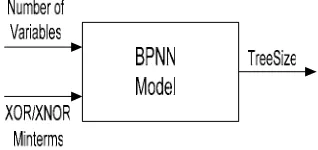
This section covers the definition and implementation of the BPNNM for modeling the XOR function complexity (Figure 5). Inputs to the model are (1) number of variables and (2) min-terms; and the output (or prediction) is the tree-size.
Figure 5. BPNNM block diagram for XOR function complexity prediction
5.1 Data Collection and Processing
[image:3.595.69.286.420.544.2]For the BPNNM in this paper, the training and validation data sets were obtained based on the experiments of section 4. Pre-processing the data sets can take a considerable amount of resources for a practical and reliably functioning BPNNM [18], [23]. In our research, the first data pre-processing step was to transform the data set in such a way that inputs have equitable distribution of importance. In other words, the larger absolute values of an input should not have more influence than the inputs with smaller magnitudes [13]. The need of such equitable distribution can be explained with Figures 6 and 7. Figure 6 shows the raw (original) data for 2 to 12 variables. Notice that the plots for 2 to 7 variables are hardly visible when all variables are plotted on the same scale. If the data were presented in its original form to the NN for training, only the 8- to 12-variable cases may be learnt by the BPNN and 2 to 7 variables values may be ignored. So in order to provide similar importance to all variable values (2 to 12), we performed pre-processing as explained in section 5.2. The data after pre-processing is plotted in Figure 7. As we can see now, the different plots (for 6-, 7-, and 8-variables) are in similar ranges which can ease the BPNN learning process.
0 50 100 150 200 250 300 350 400 450 500
1 143 285 427 569 711 853 995 1137 1279 1421 1563 1705 1847 1989
Number of XOR/XNOR Minterms
ROBDD Co
m
p
le
x
it
y
12 var
11 var
10 var
9 var 8 var
[image:3.595.313.523.579.701.2]5.2 Training and Testing the BPNNM
In order to ‘use’ or ‘run’ a trained BPNN, de-normalization and de-transformation has to be done to restore the predicted outputs to the original ranges. Steps employed in 'training' and 'running' the network is summarized here:
5.2.1 Data set
We had acquired a total of 4106 data sets (also called facts/training facts) during our simulations of XOR/XNOR functions. We used 90% of the data sets (facts) as training set and the remaining 10% as validation set.
5.2.2 Data pre-processing
We pre-processed/scaled both the horizontal and vertical axis; horizontal axis represents the min-terms (MT) and vertical axis the Tree-size (TS). Equations for MT (7) and TS (8) scaling are given below:
1 max 2 − ⋅
= v
scaled
MT MT
MT (7)
Where,
MT = original value of minterm
MTscaled = scaled value of minterm
MTmax = maximum value of minterm for all (2 to 12)
variables = 2048 V = number of variables
v scaled TS SF
TS = ⋅ (8)
Where,
TS = original value of tree-size
TSscaled = scaled value of tree-size
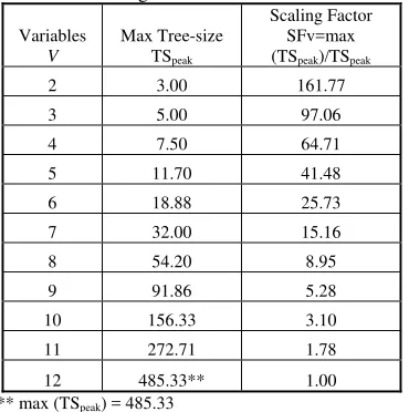
[image:4.595.313.524.83.372.2]SFv = scaling factor corresponding to variable v (listed in Table 1)
Table 1: Scaling factors for different variables
Variables V
Max Tree-size TSpeak
Scaling Factor SFv=max (TSpeak)/TSpeak
2 3.00 161.77
3 5.00 97.06
4 7.50 64.71
5 11.70 41.48
6 18.88 25.73
7 32.00 15.16
8 54.20 8.95
9 91.86 5.28
10 156.33 3.10
11 272.71 1.78
12 485.33** 1.00
** max (TSpeak) = 485.33
Effect of scaling on 2- and 3-variable data can be seen numerically in Table 2
[image:4.595.86.271.454.640.2]All variables (2 to 12) have horizontal and vertical ranges close to each other thus greatly improving the chances of NNs learning all the curves.
Table 2: Effect of pre-processing/scaling on min-terms and tree-size
ORIGINAL
VALUES SCALED VALUES Variables
v
Minterms MT
TreeSize TS
Minterms MTscaled
TreeSize TSscaled
2 0 1 0 161.77
2 1 3 1024 485.33
2 2 3 2048 485.33
3 0 1 0 97.06
3 1 4 512 388.26
3 2 4 1024 388.26
3 3 5 1536 485.33
3 4 4 2048 388.26
0 50 100 150 200 250 300 350 400 450 500
1 301 601 901 1201 1501 1801
Number of XOR/XNOR Minterms ( Scaled)
RO
BD
D Co
m
p
le
x
it
y
(
S
c
a
le
d
[image:4.595.87.269.456.639.2])
Figure 7. Scaled data (after pre-processing the raw data with equations 7 and 8) for XOR function complexity.
After the NN has been trained with the scaled data, its running/use would involve these steps:
a) Scale the input by using the equations in section 5.2.2 b) Present the scaled value to the BPNN
c) Restore to its original range the output of the BPNN to get the actual result
5.2.3 BPNNM configuration and training
In general, as the number of hidden layers increases, the prediction performance of a BPNN goes up, but this continues only up to certain extent, after which the BPNN performance starts to deteriorate [23]. To find the optimum topologies for our BPNNs, we experimented with up to 3 hidden layers; each layer consisted of a different number of neurons. Most practical problems can be modeled with one or two hidden layers [24]. However, we explored a larger design space by experimenting with a maximum of 3 hidden layers.The details of some of our BPNN’s experiments are listed in Table 3. Two neurons in the input layer correspond to two inputs, i.e., number of variables and min-terms. The single output neuron represents the model output of tree-size.
Table 3. Configuration & Training Statistics For XOR function complexity BPNN's *
CONFIGURATION TRAINING STATISTICS
No.
Input L
ayer
Neur
o
n
s
Hidden L
ayer
1 Neur
ons
Hidden L
ayer
2 Neur
ons
Hidden L
ayer
3 Neur
ons
Output Neur
ons
Facts Le
arnt
Facts Not
Learnt
% Facts
Learnt
E
pochs
1 2 3 1 3706 201 94.9% 183
2 2 4 1 3741 166 95.8% 188
3 2 5 1 3751 156 96.0% 38
4 2 7 1 3751 156 96.0% 150
5 2 10 1 3726 181 95.4% 500
6 2 3 3 1 3223 684 82.4% 500
7 2 5 5 1 3752 155 96.0% 74
8 2 7 7 3 1 3764 143 96.3% 88
9 2 3 3 5 1 3373 534 86.3% 500
10 2 5 5 5 1 3751 156 96.0% 279
* Brain Maker training parameters: Training tolerance = 0.07; testing tolerance = 0.07; learning rate adjustment type = heuristic. (See [26] for detailed explanation of these settings).
[image:5.595.313.510.113.227.2]
The matrices containing weights for different neuron layers of the chosen 2-5-1-neuron BPNN (#3) are given in Tables 4 and 5. For example, weight in ip1-h11 cell in Table 4 refers to weight between the input "ip1" and "h11" neuron of the first hidden layer. Similarly, in Table 3, the weights between the hidden and output layers are shown.
Table 4. Weight Matrix – Input Neuron Layer to Hidden Neuron Layer-1
ip1 ip2
h11 2.127 7.687
h12 6.390 -3.640
h13 -2.748 6.275
h14 3.577 -4.510
[image:5.595.312.524.472.594.2]h15 -5.157 -6.266
Table 5. Weight Matrix – Hidden Neuron Layer-1 to Output Layer
h11 h12 h13 h14 h15
op1 -5.972 -0.307 1.187 -2.991 1.544
5.3 BPNN Modeling Results and Analysis
Due to the inherent nature of NN, the input values used for running the BPNNM should be kept somewhat close to, but not necessarily the same as, the input values in the training set. Any significant deviations of the running set from the training set can provide misleading results. We used an arbitrary set of values for number of variables and number of min-terms, and used the BPNNM to predict the XOR/XNOR function complexity.
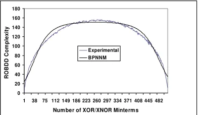
Figure 8 indicates the comparison for experimental results and BPNNM predictions of ROBDD complexity for 10
variables. It can be inferred that the BPNNM results provide a very good approximation of the ROBDD complexity.
0 20 40 60 80 100 120 140 160 180
1 38 75 112 149 186 223 260 297 334 371 408 445 482 Number of XOR/XNOR Minterms
ROBDD Co
m
p
le
x
it
y
Experimental BPNNM
Figure 8. Complexity analysis of Experimental / Neural network models for 10 variables
The same work has been repeated for Boolean functions with 2 to 15 variables. Figures 10 and 11 illustrate experimental and predicted BPNNM results for variables 8 and 12 respectively.
0 10 20 30 40 50 60
1 11 21 31 41 51 61 71 81 91 101 111 121
Number of XOR/XNOR Minterms
RO
BDD
Co
m
p
le
x
it
y
Experimental BPNNM
Figure 9. Complexity analysis of Experimental / Neural network models for 8 variables
0 100 200 300 400 500 600
1 177 353 529 705 881 1057 1233 1409 1585 1761 1937 Number of XOR/XNOR Minterms
RO
BDD
Co
mp
le
x
it
y
Experim ental BPNNM
Figure 10. Complexity analysis of Experimental / Neural network models for 12 variables
Screen capture for a sample Brain-Maker training session is shown in the Figure 11. The top part shows the training statistics, i.e. number of 'good' and 'bad' facts, tolerance, etc. ('Good' facts refer to the training sets learnt that are within specified accuracy and the 'bad' facts are outside the required accuracy). The input and output data sets are also shown near the top left of the screen. The (set of four) graphs on the bottom left show the histograms for the neuron weights in different layers whereas the graph on the bottom right shows the NN error as the training progresses.
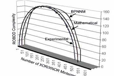
[image:5.595.74.279.476.650.2][16] for the prediction of XOR/XNOR function complexity. It can be inferred that the BPNN was able to match the experimental curve with minimum error for most of the XOR/XNOR Product terms.
Figure 11. Training the BPNN using Brain-Maker
Figure 12. Comparison with Experimental and mathematical models
6. CONCLUSION
In this research work, we have proposed a new ROBDD complexity prediction methodology based on neural network as another alternative to the CUDD simulation and the mathematical models presented by the same authors. An advantage of this model is that it is a single BPNNM for the calculation of ROBDD Complexity for different number of variables and number of XOR/XNOR minterms. Once the BPNNM is developed, it could be used to conduct further experiments with different types of inputs, in a fraction of the time what a circuit simulator would take. The results show the capabilities of training algorithms in neural networks, which produce a close match for the CUDD simulation with average errors of 0.51% for the calculation of the ROBDD complexity. In light of the results, we conclude that the proposed BPNNM in this work could be a valuable tool for exploring the complex computational capabilities of neural network. We are currently exploring the extension of this work to other complexity applications. Extending the BPNNM for wider range of variables to verify the proposed method with real benchmark circuits will also be considered.
7. REFERENCES
[1] G. E. Moore, “Progress in Digital Integrated Electronics,” IEEE IEDM, 1975, pp. 11-13.
[2] K.S. Brace, R.L. Rudell and R.E. Bryant, “Efficient implementation of a BDD package,” 27th ACM IEEE Design Automation Conference 1990. pp. 40-45. [3] I. Wegener, The Complexity of Boolean Functions,.
John Wiley and Sons Ltd, 1987
[4] C. Meinel and A. Slobodova, “On the Complexity of constructing Optimal Ordered Binary Decision diagrams,” Proc. of 19th Inter. Symposium on Mathematical Foundation of Computer Science, 1994, pp.515-524.
[5] F. Somenzi, “Efficient manipulation of decision diagrams,” Intl. J. Software Tools for Technology Transfer, (STTT), 2001, pp. 171-181.
[6] K. Priyank, “VLSI Logic Test, Validation and Verification, Properties & Applications of Binary Decision Diagrams,” Lecture Notes, Department of Electrical and Computer Engineering University of Utah, Salt Lake City, UT 84112.
[7] S. B. Akers, “Binary Decision Diagram,” IEEE Trans. Computers, Vol. 27, 1978, pp. 509-516. [8] R.E. Bryant, “Graph-based algorithm for boolean
function manipulation,” IEEE Transaction on Computers, 1986, pp. 677-691.
[9] S. Minato, Binary Decision diagrams and Applications for VLSICAD. Kluwer Academic Publishers, Dordrecht, 1995.
[10] J.E. Harlow, and F. Brglez, “Design of experiments and evaluation on of BDD ordering heuristics,” Intl. J. Software Tools for Tech. Transfer., 3: 2001, pp.193-206.
[11] K. Priyank, “VLSI Logic Test, Validation and Verification, Properties & Applications of Binary Decision Diagrams,” Lecture Notes, Department of Electrical and Computer Engineering University of Utah, Salt Lake City, UT 84112.
[12] K. Y Siu, V. P. Roychowdhury, and T. Kailath, “ Discrete Neural Computation – A theoretical Foundation,” Prentice Hall, 1995.
[13] T. Masters, Signal and Image Processing with Neural Networks, John Wiley & Sons, Inc., 1994.
[14] M. Caudill, AI Expert: Neural Network Primer, Miller Freeman Publications, 1990.
[15] I. Parberry, Circuit Complexity and Neural Networks, MIT Press, 1994.
[16] M. Raseen, P.W.C. Prasad, S.M.N.A.Senanayake, “XOR/XNOR Functional Behaviour on ROBDD Representation,” Proc. of the 14th IASTED Conference on Applied simulation and Modelling (ASM), 2005, pp. 115-119
[17] R. E. Uhrig, “Introduction to Artificial Neural Networks,” Proceedings of the 1995 IEEE IECON 21st International Conference on Industrial Electronics, Control and Instrumentation, Vol. 1, 1995, pp. 33-37.
[18] K.Yale, “Preparing the right data for training neural networks,” IEEE Spectrum, Vol. 34, Issue 3, 1997, pp. 64-66.
[19] G. Stegmayer, and O. Chiotti, “The Volterra representation of an electronic device using the Netural Network parameters,” Latin American Conference on Informatics (CLEI’2004), 2004. [20] http://www.eco.utexas.edu/faculty/Kendrick/frontpg
/NeuralNets.htm
[image:6.595.72.256.316.439.2][22] Somenzi, F. CUDD: CU Decision Diagram Package. <ftp://vlsi.colorado.edu/> pub/. 2003.
[23] J. Lawrence, “Introduction to Neural Networks – Design, Theory and Applications,” California Scientific Software Press, 1994.
[24]J. T Heaton, “Introduction to Neural Networks with Java,” Heaton Research, Inc, 2005.
[25] “Brain Maker – User’s Guide and Reference Manual, 1998,” 7th edition, California Scientific Software Press, 1998.
![Figure 1) [13]. PEs are NN equivalents of biological](https://thumb-us.123doks.com/thumbv2/123dok_es/4869955.69818/2.595.315.498.70.194/figure-pes-nn-equivalents-biological.webp)