The distributive effects of education: an unconditional quantile regression approach

(1)

C

C |

E |

_E

D |

_D

L |

_L

A |

_A

S

_S

Centro de Estudios

Distributivos, Laborales y Sociales

Maestría en Economía Facultad de Ciencias Económicas Universidad Nacional de La Plata

The Distributive Effects of Education: An

Unconditional Quantile Regression Approach

Javier Alejo, Maria Florencia Gabrielli y Walter

Sosa-Escudero

Documento de Trabajo Nro. 125

Noviembre, 2011

(2)

The Distributive Effects of Education: An Unconditional

Quantile Regression Approach

Javier Alejo

Universidad Nacional de La Plata and CONICET

Maria Florencia Gabrielli

Universidad Nacional de Cuyo and CONICET

Walter Sosa-Escudero∗

Universidad de San Andr´es and CONICET

August 30, 2011

Abstract

We use recent unconditional quantile regression methods (UQR) to study the dis-tributive effects of education in Argentina. Standard methods usually focus on mean effects, or explore distributive effects by either making stringent modeling assump-tions, and/or through counterfactual decompositions that require several temporal observations. An empirical case shows the flexibility and usefulness of UQR methods. Our application for the case of Argentina shows that education contributed positively to increased inequality in Argentina, mostly due to the effect of strongly heterogeneous effects of education on earnings.

JEL Classification: C21, I24, I31, D3

Keywords: unconditional quantile regression, income inequality, education, Ar-gentina.

∗_{Corresponding author: Walter Sosa Escudero, Departamento de Economia, Universidad de San}

(3)

1 Introduction

Considerable attention has been awarded to the effects of education on economic outcomes. The massive literature on returns to education focuses on the causal

ef-fect of increasing education (usually measured in years) on expected earnings. In

such context, a major concern of this body of research relates to the likely

endoge-nous nature of education, which biases standard OLS estimates, and usually calls

for instrumental variables strategies (See Card (2001) for a review). On the other

hand, the literature on poverty and inequality focuses on aspects of the

distribu-tion of earnings other than the mean, such as its left tail, as the case of poverty,

or its dispersion. This literature has moved gradually from unconditional analysis

(i.e., measuring income based poverty or inequality) to conditional models that help

explain the sources and causes of deprivation and/or inequality. From this perspec-tive, standard returns to education analysis is seen as one particular step (focused

on the mean) towards the final goal of quantifying the effect of the determinants of

income (including education) on the whole income distribution, and eventually on

functionals other than the mean, like poverty ratios or inequality indexes.

Regarding the goal of measuring distributional outcomes, a major step forward

relates to the increasing popularity of quantile regression (QR) methods (Koenker

(2005)), that help researchers focus on the effects of education (and other

deter-minants of income) on the whole conditional distribution, beyond the conditional

mean as in standard regression analysis. An important and recurrent result of this

literature, triggered mostly by Buchinsky (1994)’s seminal article, is that education has a markedly heterogeneous effect on the conditional distribution of income. More

concretely, several studies (see Martins and Pereira (2004)) suggest that an

addi-tional year of education has a monotonically increasing effect along the quantiles

of the conditional distribution of income. Intuitively, this implies that for higher

levels of education, the distribution of incomes is, both, shifted to the right and

more disperse; that is, education has the double impact of increasing the center and

the dispersion of the distribution of income. This previous result has lead some

researchers to worry about an undesirable, unequalizing effect of eduction, as long

as this effect translates from the conditional to the unconditional distribution of

income.

(4)

conditional distribution of incomes, even though the ultimate interest lies on the

un-conditional, marginal, distribution. The transition from conditional to unconditional

effects is not trivial. There are several approaches available. For example, Mata and

Machado (2005) propose integrating observed determinants (like education) in

con-ditional QR models, so an unconcon-ditional empirical distribution is obtained. In this

strategy, the effects of education can be quantified by integrating with respect to

alternative distributions of education and comparing resulting distributions. This

approach is similar, in spirit, to decomposition approaches (see Firpo, Fortin, and

Lemieux (2011) and Bourguignon, Lustig, and Ferreira (2004)), who try to

decom-pose observed changes in inequality (or any other distributive measure) in changes in the observed determinants, changes in the way these determinants affect income,

and usually a residual term. The nature of these decompositions depend on how

much structure is given to the model that links the distribution of incomes to that

of its observed and unobserved determinants.

In this paper we use recent advances inunconditional quantile regressions(UQR)

(Firpo, Fortin, and Lemieux (2009)) to measure the effect of education (or any other

observed determinant) on the whole (unconditional) distribution of incomes, with

minimal assumptions like those in standard Mincerian mean income analysis, and

without the need to rely on the passage of time to address the issue. That is,

unlike decomposition analysis, UQR’s allow researchers to measure the effect of a small change in education on the Gini index (or any functional of the unconditional

income distribution), in a similar sense the coefficients of a linear model capture

marginal effects on the mean in standard regression. The key analytical tool is the

recentered influence function (RIF) regression, explained in detail in section 2.

We implement this method on data for Argentina. As well documented

(Gas-parini and Cruces (2009) and Sosa Escudero and Petralia (2011, forthcoming)), in

the last 30 years Argentina went through several institutional and social episodes

that altered the distribution of incomes dramatically, which led to unusually wide

movements in poverty and inequality measures. Also, in the last 20 years the country

has experienced dramatic improvements in educational attainments, see Gasparini and Cruces (2009) for a detailed description of such changes. This scenario provides

relevant variability to explore distributive effects. To our knowledge, ours is the

first study applying an UQR strategy for this case, and, in general, this relevant

(5)

2 Standard, conditional, and unconditional quantile

re-gressions

Standard regression models are useful tools when the interest lies in measuring

the effect of a covariate on the expectation of the variable of interest. Only under

very stringent assumptions such model can be used to extrapolate the effect of

altering a covariate on other moments of the variable of interest, such as its quantiles,

its variance, or its level of inequality as measured by a standard index, like the Gini

coefficient.

In our context, the goal is to measure the effect of changes in educational levels

on the distribution of income. As a first step, and for analytic convenience and in

accordance with the natural notion of a derivative, by movements in educational

levels we mean small changes in the location of the distribution of education. Our target will be somefunctional of the distribution of income, like any quantile,

the variance, or its Gini coefficient, that is, we will be interested in a particular

feature of the distribution of income. In this sense, standard regression models

focus on the impact of education on one particular functional (the mean).

In a recent article, Firpo, Fortin, and Lemieux (2009) propose unconditional

quantile regressions as a simple way to recover such effects on the quantiles of the

unconditional distribution of a variable. In what follows we present the main ideas,

and refer to these authors for further details.

LetY be a random variable with cumulative distribution function (CDF)FY(y),

and let ν(FY) be any functional. For simplicity, we will focus on linear functionals

that can be expressed as

ν(FY) =

Z

ψ(y)dFY(y),

for some function ψ(y). For example, the mean, µY, corresponds to ψ(y) =y. In

this context, the influence function of ν atFY is given by

IF(y, FY)≡ψ(y)−

Z

ψ(y)dFY(y)

Intuitively, it measures the influence a single pointyhas on a particular functional. For example, for the mean, the influence function is given by y−µ.

It is important, to observe that

EhIF(Y, FY)

(6)

Firpo, Fortin, and Lemieux (2009), define therecentered influence function(RIF)

as

RIF(y, FY)≡IF(y, FY) +ν(FY) =ψ(y),

and, trivially,

EhRIF(Y, FY)

i

=ν(FY).

This is an important step, since, it implies that any functional of interest can be expressed as an expected value.

In order to incorporate the effect of covariates, let X be a vector of random variables. Note that, using the law of iterated expectations,

ν(FY) =

Z

RIF(y;ν)dFY(y) =

Z

EhRIF(Y;ν)|X =xidFX(x),

whereFX(x) is the marginal CDF ofX.

Suppose the distribution of X changes as a small location shift, and let α(ν) be the vector of partial effects of moving each coordinate ofX separately as a location shift. Assume also that the conditional distribution of Y given X stays constant. Then, Firpo, Fortin, and Lemieux (2009) show that theunconditional partial effect

on ν(F) of altering the CDF of X in such way is given by:

α(ν) =

Z _dE_RIF₍_y_;_ν₎_|_X₌_x

dx dF(x).

In words, this means that the partial effects of altering shifting the CDF of X

to the right (marginally) can be recovered by simple regression methods, that is, by

regressing the RIF of a Y with respect of the functional of interest, on the vector

X (the ‘RIF regression’), compute the marginal effects, and then integrate over the values ofX, as in standard regression analysis.

A relevant application for our case corresponds to the effects ofXon the uncon-ditional quantiles ofY. Let nowν(FY) =qτ denote theτ−th quantile of FY(·). Its

recentered influence function can be shown (Firpo, Fortin, and Lemieux (2009)) to

be given by

RIF(y;qτ) =qτ +IF(y;qτ) = qτ+

τ −1I{y≤qτ}

fY(qτ)

= 1I{y > qτ}

fY(qτ)

+qτ −

1−τ fY(qτ)

(7)

wherec₁,τ ≡1/fY(qτ) andc2,τ ≡qτ−c1,τ ·(1−τ). Therefore

E[RIF(Y;qτ)|X =x] = c1,τ ·E[1I{Y > qτ}|X=x] +c2,τ

= c₁,τP r[Y > qτ|X=x] +c2,τ.

This last expression is the unconditional quantile regression, that is, a regression

model that links the expected value of quantiles (as measured by the RIF) to

covari-ates. Particular specifications on P r[Y > qτ|X =x] lead to alternative regressions.

If we further assume the linear probability model P r[Y > qτ|X = x] = x′β,

trivially

β= dP r[Y > qτ|X=x]

dx .

Then, replacing in the result for the unconditional partial effect, for the case of

quantiles we get

α(ν) =c₁,τ β.

This leads to a very simple way to estimate these partial effects. Consider the

regression model

1I[y > qτ] =x′β+u.

Note that under the linear probability assumption, E(u|x) = 0. Now

1I[y > qτ]c1,τ +c2,τ = c2,τ +c1,τ x′β+u

= c2,τ +x′β∗+u,

withβ∗ _≡_c

1,τβ =α(ν). Then, ifRIF(y, qτ) =1I[y > qτ]c1,τ+c2,τ were observable,

a regression ofRIF(y, qτ) on xwould provide a consistent estimate of β∗ =α(ν).

In practice, in a first step the RIF is estimated by replacing all unknown

quan-tities by their observable counterparts. In this case, unknown quanquan-tities areqτ and

fY(qτ), which are estimated by the sampleτ−th quantile ofY, and a standard

non-parametric density estimator (e.g. kernel), respectively. The second stage regresses

the estimated RIF on xusing a standard OLS estimator.

Some remarks on this strategy are the following. First, the linear probability assumption may sound restrictive. Replacing it by a standard probit or logit

spec-ification can be easily implemented. Nevertheless, the empirical results of Firpo,

Fortin, and Lemieux (2009) indicate that results are almost indistinguishable of

those using the linear probability model, much in accordance to the recent

(8)

advocated by Angrist and Pischke (2008). Second, (asymptotic) inference in the

sec-ond stage must accommodate the fact that qτ and fY(qτ) are estimated in a first

stage. This is discussed in detail in Firpo, Fortin, and Lemieux (2009). Finally,

RIF regressions for other functionals of interest can be derived. For example, if the

functional of interest is the mean, then the RIF ofY for the mean is simplyy, then, as expected, the RIF regression is the standard regression. In our case, we will be

interested in the RIF regression for the Gini coefficient, derived in Firpo, Fortin,

and Lemieux (2009), to which we refer for details.

Finally, it is relevant to compare unconditional quantile regression with standard

quantile regressions, as defined originally by Koenker and G. (1978). The linear

quantile regression model specifies

QY|X(x, τ) =x′β(τ)

whereQY|x(τ) denotes theτ−th quantile of theconditional distribution ofY given

X=x. Consequently

β(τ) = ∂QY|X(x, τ)

∂x ,

that is, the elements of β(τ) measure the effect of altering the components of x

marginally, on theτ−th quantile of the conditional distribution ofY on X. In this model,β(τ) is understood as a non-specified function ofτ, hence its semiparametric nature.

In this context, the standard results (mentioned in the Introduction) that for the

case of education, β(τ) is a positive and monotonically increasing function means that increasing education impacts more in higher quantiles of the conditional

distri-bution of income, that is, by increasing education, all conditional quantiles move up,

but at an increasing rate along quantiles. This effect is clearly and naturally

cap-tured by quantile regressions. The ultimate effect on the unconditional distribution

(the subject of interest of distributive analysis) requires to ‘average’ these effects

ac-cording to the levels of education observed in the sample. In intuitive terms, if the

distribution ofY can be thought as factored by its conditional distribution givenX, and the marginal distribution ofX, then inequality inY represents the interaction of the inequality inX and the wayY is affected by X. Conditional quantile regres-sions can be seen as modeling the second channel, whereas unconditional quantile

regressions integrate both. For example, and as seen in the empirical part of this

(9)

be enhanced if takes place over an already unequal distribution of education, or

damped if increases in education result in a more equal distribution of education.

3 Exploring the distributive effects of education:

Ar-gentina 1992-2009

The analysis is based on micro data from Argentina’s Permanent Household

Survey (EPH) for years 1992, 1998, and 2008, for all regions available in the

pe-riod under analysis. It is worth mentioning that this survey has gone through some

methodological changes. In 1998 thirteen cities were added to the sample and be-ginning in May 2003 data collection started to be done continuously instead of twice

a year. In this respect, our results must be interpreted carefully. On the other hand,

this aspect would not be too much of a problem since our method considers only the

cross–sectional dimension of the data. However, for better comparison of our results

across time we only consider the sample that includes the cities present in the EPH

between 1992 and 1998.Cities included are: Greater La Plata, Greater Santa Fe,

Greater Paraná, Comodoro Rivadavia - Rada Tilly, Greater Córdoba, Neuquén

-Plottier Santiago del Estero - La Banda, Jujuy - Palpal´a, R´ıo Gallegos, Salta, San

Luis - El Chorrillo, Greater San Juan, Santa Rosa - Toay, Ushuaia - R´ıo Grande,

Buenos Aires City and Greater Buenos Aires. The sample considered is composed of men between 15 and 65 years old. Income is defined as the salary obtained in all

occupations measured in pesos as of December 2008.

Inequality, poverty and other aspects of the distribution of income changed

dra-matically in the last twenty years. Even though the nineties started with a period of

sustained GDP growth, the same decade witnessed a monotonic increase in

inequal-ity and poverty. The drastic crisis experienced by Argentina in 2002 led to historic

records in these measures. After that, a period of recovery followed, and inequality

and poverty decreased at a monotonic rate, reaching, in 2008, levels similar to those

observed at the beginning of the nineties. The three periods chosen for the analysis

(1992, 1998 and 2008) are representative of this behavior. For example, the Gini coefficient of hourly wages (see Table 3.1) started in 40.5, increased to 44 in 1998,

and after 2001 a period of sustained decline started and reached 39.8 in 2008. See

Gasparini and Cruces (2009) and Sosa Escudero and Petralia (2011, forthcoming)

for a complete description of these evolutions.

(10)

as measured by years of education increased from 9.9 in 1992 to 10.8 in 2008, as can

be seen in Table 3.1. A more clear picture is obtained when looking at educational

levels. For example, the proportion of individuals whose maximum level of education

is complete primary dropped from 30.3% in 1992 to 19.4%. Similarly, the same

proportion for complete high school raised from 16.4% to 22.4%. Educational levels

increased monotonically, with most of the action taking place in the center of the

distribution (around complete high school). These changes can be more drastically

appreciated in Figure 3.1, which shows the estimated densities of education for the

three periods.

In light of these results, it is natural to explore the interaction between changes in the distribution of education along those in the distribution of income. Gasparini,

Marchionni, and Sosa Escudero (2001) is the first application for Argentina that

explores this link using a microeconometric decomposition framework, and conclude

that education had equalizing effect in the period 1989–1992, and an unequalizing

effect for 1992–1998. Bustelo (2004) adopts the approach of Mata and Machado

(2005), that estimates a conditional quantile regression model from which, through

simulations, a counterfactual unconditional distribution is obtained, and finds that

that an increase in education is associated with a decrease in poverty, and a small

unequalizing effect in the period 1992–2001, with a stronger for higher levels of

education. Alejo (2006) explores the statistical significance of all these results. In this section we use RIF–regressions as introduced by Firpo, Fortin, and

Lemieux (2009) and discussed int he previous section. This approach has some

advantages, namely, (i) less data requirement since only one cross section sample

is needed, in contrast with previous work that requires repeated cross section data

with at least two periods, and the construction (by simulation) of counterfactual

distributions; (ii) RIF–regressions are easier to compute, given that in order to

re-cover the marginal distribution of income it is not necessary to use a large number

of simulations as in Mata and Machado (2005) or other numerical solutions (e.g.

Melly (2005)); finally, (iii) the marginal effects can be directly interpreted from the

estimation results.

As discussed in the previous section, we estimate RIF regressions for several

unconditional quantiles, using a linear probability specification. We also estimate a

RIF regression for the Gini coefficient. We use the usual covariates in standard

(11)

to control for regional effects.

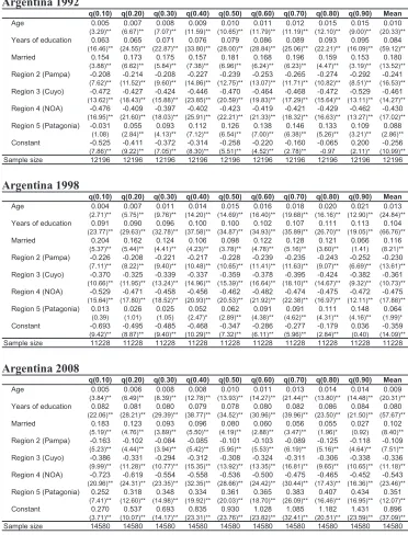
As a previous step, Table 3.2 presents a conditional quantile regression analysis

for quantiles ranging from 0.1 to 0.9. The last column of this table presents results

of a standard OLS regression. Tables 3.3 presents results based on unconditional

quantile regression, and the last columns shows results for the RIF regression of

the Gini coefficient. For convenience, estimated coefficients for these two tables are

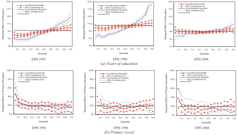
represented in the first row of graphics in Figure 3.2

Consider the first graph of Figure 3.2, which represents the estimated

coeffi-cients of years education for the conditional and unconditional quantile regressions

in Table 3.2, for 1992. The horizontal line represents the ‘mean’ effect associated to the standard OLS estimator, 0.084, in this case. Were education set exogenously,

this implies that an extra year of education led to an increase of around 8.4% in

ex-pected wages. The solid line with triangles represent conditional quantile regression

estimates, and the solid line (with no ticks), represents estimates for unconditional

quantiles.

A first interesting fact is that, consistently with most previous results, effects are

heterogeneous and increasing along the quantiles. CQR results suggest that effects

range from 0.063 for the first decile to 0.095 to the 9th decile of the conditional

distribution of wages. As stressed in the Introduction, this result must be interpreted

carefully. It only suggest that after controlling for all covariates, all quantiles of the conditional distribution increase when education is enhanced, but at an increasing

rate the higher the quantiles. A common difficulty associated with interpreting these

results is that the top (bottom) of the conditional distribution does not coincide

with the top (bottom) of its unconditional counterpart. That is, the positive and

heterogeneous CQR effects do not imply that education has a stronger effect for the,

say, rich, but for the ‘conditionally’ rich, that is, after controlling for all covariates.

Consequently, within the CQR it is difficult to see if this unequalizing effect

translates to the unconditional distribution of incomes, hence the usefulness of the

UQR approach, that studies effect directly on the distribution of income.

Remark-ably, UQR results show an even more pronounced heterogeneous behavior, with effect ranging from 0.046 to 0.140. UQR results are more directly interpretable

since, now they suggest that the effects of education are stronger for the rich.

Dif-ferences between the CQR and the UQR approach might be due to the fact that the

(12)

already unequal (and markedly asymmetric) distribution of education of 1992. As

stressed in the previous sections, and unlike CQR, UQR integrates the heterogenous

effects on the conditional distribution with the existing levels of education, leading

to an enhanced heterogenous effect.

Finally, RIF regressions results for the Gini coefficient (last column of Table

3.3) are interesting. First, in order to obtain comparable results, the regression is

estimated using levels of wages, not logs as in standard Mincer equations. Hence,

results suggest that shifting the distribution of education marginally, leads to an

unequalizing increase of 1.83 points in the Gini coefficient. At this point it is

inter-esting to remark that, qualitatively and quantitatively, these results are in agreement with those found by alternative methods (Gasparini, Marchionni, and Sosa

Escud-ero (2001) andBustelo (2004)). A major advantage is that the UQR requires cross

sectional information only, like in standard Mincer equations, and unlike previous

results who require either two points in time or the construction of counterfactual

distributions by simulation.

We then explore these effects for the remaining two periods (1998 and 2002).

First, in 1998 all effects move to the right, for example, the mean effect moves from

0.084 in 1992 to 0.104. Interestingly, the CQR results, though still positive and

increasing along the quantiles of the conditional distribution, are less disperse, with

a difference now less than 0.02 points between the 0.1 and the 0.9 decile, suggesting a decreasing unequalizing effect. On the contrary, UQR results are markedly more

heterogeneous, ranging from 0.066 to 0.19 along the quantiles of the unconditional

distribution of wages, suggesting a strong unequalizing effect of education through

this channel. This coincides with the beginning of the worst part of the performance

in inequality in the period under analysis. This effect is further confirmed by the

corresponding coefficient for education in the RIF regression for the Gini coefficient,

which now leads to an increase of almost 2 points. It is important to remark that

beyond the qualitative or statistical relevance of this figure, in economic terms, 2

points along the Gini coefficient of Argentina is a large figure, mostly from the

perspective that the swings in inequality in the period under analysis range around 4 points.

The year 2008 presents a completely different picture. The levels of the effects

are now similar to those of 1992, but the heterogeneity reduced drastically, as can be

(13)

stable around the mean effect (0.08), while UQR effect now range from 0.063 to

0.11. The effect of education on the Gini index is still unequalizing, but considerably

smaller (0.49 in 2008).

Even though it seems reasonable to measure the amount of human capital by

years of formal education, this information is sometimes not considered as a

sat-isfactory or adequate measure of qualification in the labor market and as a result

the reference taken is if the worker has finished certain level of education. This is

known in the literature as “sheepskin effects” (Hungerford and Solon (1987)). To

this purpose we run the same regressions as before but now replacing years of

edu-cation with binary variables indicating the highest level of eduedu-cation reached by the individual. The results (OLS and QR) for the conditional distribution are reported

in Table 3.4. Table 3.5 shows the results for the unconditional distribution (RIF–

regressions). In both cases the base category is unfinished primary school. Results

are shown graphically as before, in the 2nd to 4th row of graphs in Figure 3.2.

Finishing primary school has a positive but homogeneous effect on both the

con-ditional and unconcon-ditional distribution of income, along the whole period. Moreover,

as measured by the RIF/Gini regression, this step induces an overallequalizingeffect

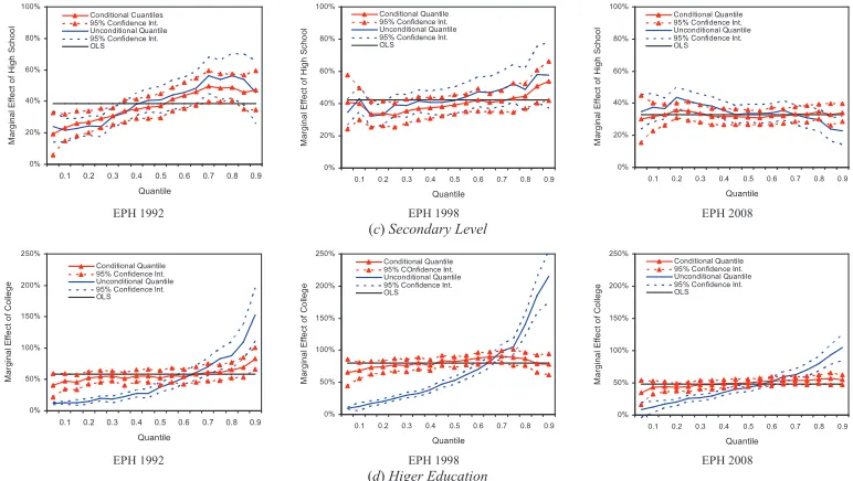
of education on the distribution of income. Moving to other levels, the heterogeneity

starts to increase and now follows a pattern closer to that found when measuring

education in years: heterogeneity in effects is important but dampens in 2008. Also, it is interesting to see that higher education (as compared to the base category),

shows a highly heterogeneous performance that peaked in 1998, coinciding with

the period where inequality peaked in Argentina, suggesting that education had a

markedly different effect which fueled inequality up.

4 Concluding remarks

Even though abundant literature exists on the effect of education on expected

earnings, distributive effects are more difficult to assess an quantify. This paper

shows that unconditional quantile regression analysis is a powerful and simple tool to characterize changes in inequality and, in general, in other aspects of the distribution

of income, like its quantiles. RIF regressions exploit cross-sectional variability and

can be easily reproduced over time to measure the evolution of these effects.

The case of Argentina is a very relevant one, in light of the drastic movements in

(14)

In line with existing results for several countries and periods (including Argentina),

the conditional quantile regression results in this paper suggest, indeed, the presence

of an unequalizing effect of education through positive and heterogeneous returns,

increasing along the quantiles of the conditional distribution, a particularly strong

effect for the nineties. Our unconditional quantile regression results suggest that

in the nineties these heterogeneous returns were further enhanced and co-moved

positively with the observed increases in inequality, as measured by the Gini index.

Interestingly, results for the year 2008 suggest that these unequalizing effects

re-duced dramatically, revitalizing the role of education as a powerful policy variable

to improve welfare. To summarize, the rapid increase in inequality in the nineties coincided with a period of increased education, particularly successful in moving

individuals into high school, and a markedly heterogeneous performance in terms

of how discrepancies in education were remunerated in the market. That is, in this

period, the strong unequalizing effect of education is not due to increased

educa-tion per-se, but on discrepancies in either quality of educaeduca-tion, the way the market

remunerates these discrepancies, and the interaction with abilities and their own

remunerations. The results for the end of the nineties, suggest that this strong

un-equalizing effect has disappeared, reaffirming the relevant role fostering education

has on improving welfare. Another relevant result, that reinforces the previous

re-sult, is that the channel that increases inequality through heterogeneity is almost absent when education increases at the lowest levels.

Finally, this paper refrains from exploring the effect of treating education as an

endogenous variable. Unlike mean results, methods for handling such problem when

the interest lies in distributive effects are still in their infancy (Powell (2011)), and,

surely, are a top priority for further work. Nevertheless, it is relevant to remark

that it is not clear ex–ante that the concerns that affect mean estimates translate

into other functionals alike. For example, when the interest lies in inequality, a

biased counterfactual distribution that arises by ignoring endogeneities does not

necessarily biased the functionals of interest for distributive purposes. For example,

if neglected endogeneities bias the whole conditional distribution up (or down), this affects negatively the estimation of the mean effect, but not necessarily that

of distributive effects, which depend on distances between quantiles and not on

their levels. A detailed exploration of these effects is a relevant route for further

(15)

(16)

References

Alejo, J. (2006): “Desigualdad salarial en el gran Buenos Aires: una aplicaci´on

de regresi´on por cuantiles en microdescomposiciones,” Documento de Trabajo,

CEDLAS, UNLP, Argentina., (36).

Angrist, J., and J.-S. Pischke (2008): Mostly Harmless Econometrics:An

Em-piricist’s Companion. Princeton University Press, 1 edition edn.

Bourguignon, F., N. Lustig, andF. Ferreira(2004): The Microeconomics of

Income Distribution Dynamics. Oxford University Press, Washington.

Buchinsky, M.(1994): “Changes in the U.S. Wage Structure 1963-1987:

Applica-tion of Quantile Regression,” Econometrica, 62(2), 405–458.

Bustelo, M. (2004): “Caracterizaci´on de los Cambios en la Desigualdad y la

Pobreza en Argentina Haciendo Uso de T´enicas de Descomposiciones

Microe-conom´etricas,”CEDLAS, Documento de Trabajo, (13).

Card, D. (2001): “Estimating the Return to Schooling: Progress on Some

Persis-tent Econometric Problems,” Econometrica, 69, 1127–1160.

Firpo, S., N. Fortin, and T. Lemieux(2009): “Unconditional Quantile

Regres-sions,” Econometrica, 77(3), 953–973.

(2011): Handbook of Labor Economicschap. Decomposition Method in

Economics. Elsevier, in press.

Gasparini, L., andG. Cruces(2009): “Desigualdad En Argentina: Una Revisi´on

De La Evidencia Emp´ırica,” Desarrollo Economico, 1.

Gasparini, L., M. Marchionni, and W. Sosa Escudero (2001): Distribuci´on

del Ingreso en la Argentina: Perspectivas y Efectos sobre el Bienestar. Premio

Fulvio S. Pagani, Fundacin Arcor.

Hungerford, T., and G. Solon (1987): “Sheepskin effects in the returns to

education,” The Review of Economics and Statistics, 69(1), 175–177.

Koenker, R. (2005): Quantile Regression. Cambridge University Press,

(17)

Koenker, R., and B. G. (1978): “Regression Quantiles,” Econometrica, 46(1),

33–50.

Martins, P., andP. Pereira(2004): “Does Education Reduce Wage Inequality?

Quantile Regression Evidence from 16 Countries,”Labour Economics, 11(3), 355–

371.

Mata, J., and J. Machado(2005): “Counterfactual decomposition of changes in

wage distributions using quantile regression,” Journal of Applied Econometrics,

20(445-465).

Melly, B. (2005): “Decomposition of Differences in Distribution Using Quanitle

Regressions,” Labour Economics, 12, 577–90.

Powell, D.(2011): “Unconditional Quantile Regression for Exogenous or

Endoge-nous Treatment Variables,” Labor and Population working paper series,

(WR-824).

Sosa Escudero, W., and S. Petralia (2011, forthcoming): Comparartive

Growth and Development: Brazil and Argentinachap. I Can Hear the Grass Grow:

(18)

[image:18.612.130.483.151.415.2]

Tables and Figures

Table 3.1: Summary statistics of survey data. Argentina 1992 - 2008 Sample: Men between 16 and 64 years old

Year

Mean Std. Dev. Quantile 0.10 Median Quantile 0.90 Range 90-10

1992 11.5 12.0 4.1 8.2 21.6 17.5

1998 12.6 14.3 3.8 8.6 25.7 21.9

2008 11.4 15.9 3.6 8.7 21.1 17.5

1992 36.6 13.1 20 36 56 36

1998 37.4 12.3 22 36 55 33

2008 36.5 13.6 19 35 56 37

1992 9.9 3.8 7 10 15 8

1998 10.0 3.8 7 10 16 9

2008 10.8 3.7 7 12 16 9

Prim. incom. Prim. compl. Dropouts Highschool Coll. incom. Coll. compl.

1992 9.3% 30.3% 24.5% 16.4% 11.4% 8.1%

1998 7.6% 27.4% 24.7% 18.0% 11.4% 10.7%

2008 6.9% 19.4% 23.8% 22.4% 14.8% 12.7%

GBA Pampa Cuyo NOA Patagonia Total

1992 65.9% 20.7% 3.5% 6.2% 3.7% 100%

1998 73.8% 14.4% 3.2% 5.2% 3.4% 100%

2008 70.7% 16.6% 3.3% 6.0% 3.4% 100%

Educational Level

Region Variable

Hourly wage

Age

Year of education

(19)

[image:19.612.118.490.160.648.2]

Table 3.2 marginal effects on conditional wage distributions: Quantile Regression -Men between 16 and 64 years old

Argentina 1992

q(0.10) q(0.20) q(0.30) q(0.40) q(0.50) q(0.60) q(0.70) q(0.80) q(0.90) Mean

Age 0.005 0.007 0.008 0.009 0.010 0.011 0.012 0.015 0.015 0.010

(3.29)** (6.67)** (7.07)** (11.59)** (10.65)** (11.79)** (11.19)** (12.10)** (9.00)** (20.33)**

Years of education 0.063 0.065 0.071 0.076 0.079 0.086 0.089 0.093 0.095 0.084

(16.46)** (24.55)** (22.87)** (33.80)** (28.00)** (28.84)** (25.06)** (22.21)** (16.09)** (59.12)**

Married 0.154 0.173 0.175 0.157 0.181 0.168 0.196 0.159 0.153 0.180

(3.88)** (6.62)** (5.84)** (7.38)** (6.96)** (6.24)** (6.23)** (4.47)** (3.19)** (13.52)**

Region 2 (Pampa) -0.208 -0.214 -0.208 -0.227 -0.239 -0.253 -0.265 -0.274 -0.292 -0.241

(7.62)** (11.52)** (9.60)** (14.86)** (12.75)** (13.07)** (11.71)** (10.82)** (8.51)** (16.53)**

Region 3 (Cuyo) -0.472 -0.427 -0.424 -0.446 -0.470 -0.464 -0.468 -0.472 -0.529 -0.461

(13.62)** (18.43)** (15.88)** (23.85)** (20.59)** (19.83)** (17.29)** (15.64)** (13.11)** (14.27)**

Region 4 (NOA) -0.476 -0.409 -0.397 -0.402 -0.423 -0.419 -0.421 -0.429 -0.462 -0.430

(16.95)** (21.60)** (18.03)** (25.91)** (22.21)** (21.33)** (18.32)** (16.63)** (13.27)** (17.02)**

Region 5 (Patagonia) -0.031 0.055 0.093 0.112 0.126 0.138 0.146 0.133 0.109 0.088

(1.08) (2.84)** (4.13)** (7.12)** (6.54)** (7.00)** (6.38)** (5.26)** (3.21)** (2.86)**

Constant -0.525 -0.411 -0.372 -0.314 -0.258 -0.220 -0.160 -0.065 0.200 -0.256

(7.86)** (9.22)** (7.05)** (8.30)** (5.51)** (4.52)** (2.78)** -0.97 (2.11)* (10.99)**

Sample size 12196 12196 12196 12196 12196 12196 12196 12196 12196 12196

Argentina 1998

q(0.10) q(0.20) q(0.30) q(0.40) q(0.50) q(0.60) q(0.70) q(0.80) q(0.90) Mean

Age 0.004 0.007 0.011 0.014 0.015 0.016 0.018 0.020 0.021 0.013

(2.71)** (5.75)** (9.76)** (14.20)** (14.69)** (16.40)** (19.68)** (16.16)** (12.90)** (24.84)**

(23.77)** (29.63)** (32.78)** (37.58)** (34.87)** (34.93)** (35.89)** (26.70)** (19.05)** (66.76)**

Married 0.204 0.162 0.124 0.106 0.098 0.122 0.128 0.121 0.066 0.116

(5.37)** (5.44)** (4.41)** (4.23)** (3.78)** (4.78)** (5.16)** (3.60)** (1.41) (8.21)**

Region 2 (Pampa) -0.226 -0.208 -0.221 -0.217 -0.228 -0.239 -0.235 -0.243 -0.252 -0.230

(7.11)** (8.22)** (9.40)** (10.48)** (10.65)** (11.41)** (11.63)** (9.07)** (6.69)** (13.61)**

Region 3 (Cuyo) -0.370 -0.325 -0.339 -0.337 -0.359 -0.378 -0.395 -0.424 -0.382 -0.361

(10.66)** (11.95)** (13.24)** (14.96)** (15.39)** (16.64)** (18.10)** (14.67)** (9.32)** (10.73)**

Region 4 (NOA) -0.529 -0.471 -0.458 -0.456 -0.462 -0.482 -0.474 -0.475 -0.472 -0.475

(15.64)** (17.80)** (18.52)** (20.93)** (20.53)** (21.92)** (22.38)** (16.97)** (12.11)** (17.88)**

Region 5 (Patagonia) 0.013 0.026 0.025 0.052 0.062 0.091 0.091 0.111 0.148 0.064

(0.39) (1.01) (1.05) (2.47)* (2.89)** (4.38)** (4.62)** (4.31)** (4.16)** (1.99)*

Constant -0.693 -0.495 -0.485 -0.468 -0.347 -0.286 -0.277 -0.179 0.036 -0.359

(9.42)** (8.87)** (9.40)** (10.29)** (7.32)** (6.11)** (5.96)** (2.84)** (0.40) (14.09)**

Sample size 11228 11228 11228 11228 11228 11228 11228 11228 11228 11228

Argentina 2008

q(0.10) q(0.20) q(0.30) q(0.40) q(0.50) q(0.60) q(0.70) q(0.80) q(0.90) Mean

Age 0.005 0.006 0.008 0.008 0.010 0.011 0.013 0.014 0.014 0.009

(3.84)** (6.49)** (8.39)** (12.78)** (13.93)** (14.27)** (21.44)** (13.80)** (14.48)** (20.31)**

(22.06)** (28.21)** (29.39)** (38.77)** (34.52)** (30.96)** (39.96)** (23.50)** (21.50)** (57.67)**

Married 0.183 0.123 0.093 0.096 0.080 0.060 0.056 0.055 0.027 0.102

(5.19)** (4.76)** (3.89)** (5.50)** (4.19)** (2.88)** (3.47)** (1.96)* (0.92) (8.40)**

Region 2 (Pampa) -0.163 -0.102 -0.084 -0.085 -0.101 -0.103 -0.089 -0.125 -0.118 -0.109

(5.23)** (4.44)** (3.94)** (5.42)** (5.95)** (5.53)** (6.19)** (5.16)** (4.64)** (7.51)**

Region 3 (Cuyo) -0.386 -0.331 -0.294 -0.312 -0.308 -0.324 -0.311 -0.306 -0.338 -0.336

(9.99)** (11.28)** (10.77)** (15.35)** (13.92)** (13.35)** (16.81)** (9.65)** (10.65)** (11.18)**

Region 4 (NOA) -0.723 -0.619 -0.554 -0.558 -0.536 -0.500 -0.475 -0.465 -0.452 -0.543

(20.96)** (24.31)** (23.35)** (32.35)** (28.66)** (24.42)** (30.44)** (17.43)** (16.36)** (23.46)**

(7.41)** (12.60)** (14.98)** (19.92)** (20.03)** (18.70)** (26.09)** (16.46)** (16.95)** (12.07)**

Constant 0.270 0.537 0.693 0.835 0.930 1.028 1.085 1.182 1.431 0.896

(3.71)** (10.07)** (14.17)** (23.31)** (23.76)** (23.82)** (32.41)** (20.51)** (23.59)** (37.09)**

Sample size 14580 14580 14580 14580 14580 14580 14580 14580 14580 14580

(20)

[image:20.612.127.478.146.663.2]

Table 3.3: Marginal effects on marginal wage distribution RIF Regression - Men between 16 and 64 years old

Argentina 1992

q(0.10) q(0.20) q(0.30) q(0.40) q(0.50) q(0.60) q(0.70) q(0.80) q(0.90) Gini

Indicator 4.64 5.81 6.83 7.89 9.32 10.92 13.26 17.06 24.52 40.5

Marginal Effects

Age 0.005 0.006 0.008 0.009 0.010 0.012 0.013 0.014 0.016 0.14

(3.16)** (5.69)** (7.54)** (8.77)** (8.37)** (10.12)** (9.59)** (8.43)** (6.89)** (3.86)**

(13.23)** (17.39)** (20.81)** (23.46)** (24.44)** (25.81)** (27.15)** (23.58)** (15.89)** (17.07)**

Married 0.149 0.168 0.142 0.134 0.170 0.172 0.213 0.205 0.197 2.05

(4.02)** (5.85)** (5.18)** (4.58)** (5.44)** (5.14)** (5.68)** (4.70)** (3.22)** (2.03)*

Region 2 (Pampa) -0.244 -0.213 -0.216 -0.236 -0.253 -0.256 -0.255 -0.260 -0.268 -0.76

(8.99)** (10.28)** (11.03)** (11.55)** (11.53)** (10.94)** (9.64)** (8.55)** (6.16)** (0.68)

Region 3 (Cuyo) -0.667 -0.550 -0.469 -0.453 -0.428 -0.414 -0.394 -0.386 -0.341 5.85

(14.98)** (19.06)** (18.89)** (18.70)** (16.98)** (16.08)** (13.90)** (12.64)** (8.11)** (2.38)*

Region 4 (NOA) -0.614 -0.467 -0.423 -0.398 -0.398 -0.368 -0.366 -0.344 -0.337 4.11

(18.43)** (20.27)** (20.44)** (18.95)** (18.25)** (16.05)** (14.62)** (12.26)** (8.78)** (2.14)*

Region 5 (Patagonia) -0.045 0.022 0.067 0.113 0.131 0.163 0.191 0.219 0.125 -0.18

(1.65) (1.08) (3.37)** (5.32)** (5.64)** (6.53)** (6.77)** (6.72)** (2.78)** (0.08)

Constant -0.407 -0.272 -0.214 -0.245 -0.221 -0.293 -0.343 -0.202 -0.165 0.15

(5.74)** (5.04)** (4.27)** (4.78)** (4.12)** (5.30)** (5.96)** (2.94)** (1.49) (8.66)**

Sample size 12196 12196 12196 12196 12196 12196 12196 12196 12196 12196

Argentina 1998

q(0.10) q(0.20) q(0.30) q(0.40) q(0.50) q(0.60) q(0.70) q(0.80) q(0.90) Gini

Indicator 4.29 5.66 6.9 8.08 9.73 11.66 14.14 18.28 29.16 44.0

Marginal Effects

Age 0.005 0.007 0.010 0.011 0.012 0.014 0.016 0.019 0.024 0.35

(2.74)** (5.87)** (8.42)** (9.38)** (10.21)** (11.61)** (12.60)** (12.19)** (9.51)** (9.23)**

(14.50)** (19.87)** (24.91)** (29.23)** (31.53)** (33.87)** (35.15)** (30.45)** (20.08)** (18.02)**

Married 0.238 0.144 0.112 0.120 0.117 0.104 0.072 0.108 0.063 -4.00

(5.34)** (4.78)** (3.86)** (4.22)** (3.93)** (3.38)** (2.12)* (2.65)** (0.97) (3.99)**

Region 2 (Pampa) -0.143 -0.155 -0.192 -0.219 -0.228 -0.235 -0.243 -0.261 -0.421 -4.25

(3.99)** (6.16)** (7.94)** (9.46)** (9.50)** (9.49)** (8.81)** (7.79)** (8.54)** (3.55)**

Region 3 (Cuyo) -0.501 -0.365 -0.391 -0.379 -0.371 -0.331 -0.304 -0.292 -0.355 2.08

(10.26)** (12.17)** (14.53)** (15.25)** (14.75)** (12.98)** (11.00)** (8.87)** (7.22)** (0.88)

Region 4 (NOA) -0.794 -0.545 -0.520 -0.436 -0.432 -0.411 -0.372 -0.343 -0.453 3.42

(15.86)** (18.51)** (20.11)** (18.23)** (17.92)** (17.06)** (14.19)** (10.96)** (10.02)** (1.82)

(0.19) (0.73) (1.14) (2.71)** (3.27)** (3.72)** (4.44)** (4.05)** (1.18) (0.04)

Constant -0.597 -0.278 -0.265 -0.237 -0.200 -0.239 -0.339 -0.435 -0.527 0.14

(6.48)** (4.62)** (4.85)** (4.74)** (3.98)** (4.89)** (6.45)** (6.62)** (4.30)** (7.73)**

Sample size 11228 11228 11228 11228 11228 11228 11228 11228 11228 11228

Argentina 2008

q(0.10) q(0.20) q(0.30) q(0.40) q(0.50) q(0.60) q(0.70) q(0.80) q(0.90) Gini

Indicator 3.62 4.97 6.21 7.37 8.69 10.14 12.28 15.35 21.12 39.8

Marginal Effects

Age 0.005 0.006 0.008 0.009 0.010 0.011 0.012 0.013 0.015 0.18

(2.87)** (5.68)** (8.50)** (10.76)** (12.44)** (13.23)** (13.24)** (12.65)** (10.18)** (3.39)**

(13.46)** (21.14)** (26.65)** (31.17)** (33.46)** (33.71)** (31.84)** (26.63)** (19.25)** (3.04)**

Married 0.276 0.136 0.071 0.070 0.066 0.062 0.054 0.010 0.046 -0.56

(6.52)** (4.69)** (2.97)** (3.14)** (3.06)** (2.76)** (2.24)* (0.36) (1.19) (0.40)

Region 2 (Pampa) -0.114 -0.087 -0.118 -0.112 -0.096 -0.094 -0.091 -0.090 -0.162 -2.50

(3.21)** (3.47)** (5.51)** (5.65)** (4.94)** (4.65)** (4.19)** (3.44)** (4.61)** (1.49)

Region 3 (Cuyo) -0.430 -0.420 -0.372 -0.305 -0.289 -0.284 -0.312 -0.292 -0.311 1.14

(7.94)** (11.27)** (12.64)** (11.63)** (11.86)** (11.64)** (12.74)** (10.67)** (9.28)** (0.33)

Region 4 (NOA) -1.000 -0.714 -0.587 -0.484 -0.431 -0.385 -0.371 -0.354 -0.336 7.66

(18.56)** (22.25)** (23.99)** (22.78)** (21.89)** (19.55)** (18.39)** (15.44)** (11.21)** (2.87)**

(5.36)** (10.23)** (12.48)** (15.39)** (16.28)** (18.33)** (17.30)** (16.19)** (12.39)** (1.10)

Constant 0.330 0.558 0.753 0.823 0.924 0.999 1.131 1.182 1.291 0.28

(3.43)** (8.68)** (14.75)** (18.43)** (22.81)** (24.40)** (25.84)** (21.30)** (16.51)** (9.91)**

Sample size 14580 14580 14580 14580 14580 14580 14580 14580 14580 14580

(21)

[image:21.612.151.461.281.537.2]

Table 3.4: Marginal effects of education on conditional wage distribution Quantile Regression - Men between 16 and 64 years old

Argentina 1992

Argentina 1998

Argentina 2008

Source: own calculations based on SEDLAC (CEDLAS and World Bank). Note: years old, marital status and regional dummies also was included in regression

q(0.10) q(0.20) q(0.30) q(0.40) q(0.50) q(0.60) q(0.70) q(0.80) q(0.90) Media

Primary complete 0.266 0.223 0.190 0.188 0.179 0.152 0.116 0.143 0.164 0.21 (5.67)** (5.79)** (6.28)** (5.58)** (4.31)** (3.44)** (2.18)* (3.17)** (2.63)** (9.83)** Secondary incomplete 0.353 0.319 0.304 0.338 0.310 0.312 0.308 0.362 0.401 0.36

(7.09)** (7.90)** (9.55)** (9.57)** (7.09)** (6.69)** (5.48)** (7.48)** (5.98)** (16.31)** Secondary complete 0.499 0.492 0.496 0.539 0.551 0.589 0.610 0.633 0.635 0.59

(9.69)** (11.76)** (15.02)** (14.67)** (12.08)** (12.13)** (10.41)** (12.60)** (9.05)** (25.77)** College incomplete 0.640 0.669 0.694 0.757 0.758 0.798 0.806 0.892 0.956 0.81

(10.68)** (13.97)** (18.35)** (17.90)** (14.38)** (14.15)** (11.81)** (15.31)** (11.99)** (31.00)** College complete 0.968 1.019 1.052 1.098 1.079 1.130 1.224 1.282 1.465 1.18

(16.10)** (20.77)** (26.78)** (25.15)** (19.96)** (19.70)** (17.71)** (21.73)** (17.73)** (44.48)** Sample size 10618 10618 10618 10618 10618 10618 10618 10618 10618 10618

q(0.10) q(0.20) q(0.30) q(0.40) q(0.50) q(0.60) q(0.70) q(0.80) q(0.90) Media

Primary complete 0.212 0.137 0.185 0.148 0.142 0.166 0.215 0.230 0.213 0.19 (3.40)** (2.93)** (3.99)** (3.68)** (3.89)** (3.95)** (5.42)** (5.00)** (2.96)** (8.02)** Secondary incomplete 0.371 0.270 0.298 0.291 0.307 0.354 0.389 0.406 0.384 0.36

(18.38)** (22.69)** (24.26)** (27.51)** (31.68)** (29.44)** (32.33)** (27.92)** (17.62)** (51.67)** Sample size 11231 11231 11231 11231 11231 11231 11231 11231 11231 11231

q(0.10) q(0.20) q(0.30) q(0.40) q(0.50) q(0.60) q(0.70) q(0.80) q(0.90) Media

Primary complete 0.212 0.156 0.134 0.122 0.137 0.186 0.190 0.220 0.195 0.19 (3.11)** (4.06)** (2.93)** (2.87)** (3.27)** (3.94)** (4.63)** (5.18)** (3.68)** (8.14)** Secondary incomplete 0.238 0.215 0.227 0.245 0.262 0.345 0.348 0.366 0.350 0.30

(22)

Table 3.5: Marginal effects of education on unconditional wage distribution RIF Regression - Men between 16 and 64 years old

Argentina 1992

q(0.10) q(0.20) q(0.30) q(0.40) q(0.50) q(0.60) q(0.70) q(0.80) q(0.90) Gini

Indicator 4.09 5.12 6.02 6.96 8.21 9.63 11.69 15.04 21.61 40.5

Marginal Effects

Primary complete 0.280 0.217 0.165 0.149 0.169 0.168 0.174 0.188 0.145 -3.26

(4.10)** (4.29)** (3.52)** (3.13)** (3.49)** (3.47)** (3.72)** (4.55)** (2.95)** (2.06)*

Secondary incomplete 0.339 0.320 0.302 0.299 0.344 0.354 0.380 0.432 0.307 -2.10

(4.83)** (6.15)** (6.28)** (5.99)** (6.73)** (6.80)** (7.28)** (8.47)** (5.02)** (1.26)

Secondary complete 0.497 0.462 0.466 0.532 0.580 0.626 0.739 0.752 0.601 -1.42

(7.27)** (9.09)** (9.81)** (10.78)** (11.09)** (11.47)** (12.79)** (12.36)** (7.30)** (0.82)

College incomplete 0.600 0.577 0.613 0.685 0.786 0.875 0.981 1.078 1.108 2.07

(8.54)** (10.84)** (12.42)** (12.79)** (13.63)** (13.92)** (14.01)** (13.14)** (8.79)** (1.06)

College complete 0.625 0.611 0.652 0.806 0.956 1.151 1.437 1.632 2.133 37.08

(9.85)** (12.56)** (14.14)** (16.94)** (18.51)** (20.73)** (22.61)** (19.49)** (13.56)** (18.64)**

Sample size 10618 10618 10618 10618 10618 10618 10618 10618 10618 10618

Argentina 1998

q(0.10) q(0.20) q(0.30) q(0.40) q(0.50) q(0.60) q(0.70) q(0.80) q(0.90) Gini

Indicator 3.78 4.99 6.08 7.12 8.57 10.27 12.46 16.11 25.7 44.0

Marginal Effects

(2.76)** (2.97)** (2.43)* (3.19)** (3.49)** (3.28)** (3.87)** (3.87)** (2.87)** (0.78)

(4.55)** (4.93)** (5.46)** (6.16)** (6.14)** (6.82)** (7.01)** (7.44)** (5.34)** (0.85)

(7.57)** (8.56)** (9.38)** (10.86)** (11.12)** (11.79)** (11.98)** (10.86)** (8.40)** (1.79)

College incomplete 0.852 0.716 0.799 0.871 0.949 1.017 1.100 1.155 0.948 -2.47

(9.02)** (11.84)** (14.26)** (16.15)** (16.78)** (17.44)** (16.89)** (14.71)** (8.40)** (1.29)

(9.06)** (12.59)** (15.79)** (19.76)** (22.73)** (26.86)** (29.97)** (27.95)** (19.15)** (19.62)**

Sample size 11231 11231 11231 11231 11231 11231 11231 11231 11231 11231

Argentina 2008

q(0.10) q(0.20) q(0.30) q(0.40) q(0.50) q(0.60) q(0.70) q(0.80) q(0.90) Gini

Indicator 3.62 4.97 6.21 7.37 8.69 10.14 12.28 15.35 21.12 39.8

Marginal Effects

(2.46)* (2.80)** (3.26)** (4.26)** (4.24)** (3.64)** (3.18)** (1.92) (2.15)* (0.69)

(2.52)* (4.36)** (5.09)** (7.01)** (7.17)** (6.95)** (6.39)** (4.41)** (5.09)** (0.69)

(6.48)** (9.00)** (10.30)** (11.81)** (12.10)** (11.52)** (10.54)** (7.44)** (6.90)** (1.12)

College incomplete 0.821 0.873 0.849 0.864 0.822 0.793 0.724 0.715 0.750 -5.70

(8.44)** (12.13)** (14.77)** (17.53)** (17.93)** (16.71)** (14.32)** (11.43)** (10.40)** (1.92)

(7.79)** (11.97)** (15.33)** (19.72)** (21.95)** (23.10)** (23.01)** (19.08)** (17.06)** (2.46)*

Sample size 14608 14608 14608 14608 14608 14608 14608 14608 14608 14608

(23)

[image:23.612.151.467.124.373.2]

Figure 3.1: Wage marginal distribution. Argentina 1992 - 2008 Sample: Men between 16 and 64 years old

0 .2 .4 .6 D e n s it y

-2 0 2 4 6

Wage (log)

2008 1998

1992

Source: own calculations based on SEDLAC (CEDLAS and World Bank).

Figure 3.2: Marginal effects of education on unconditional wage distribution - Men between 16 and 64 years old

2% 5% 8% 11% 14% 17% 20%

0.1 0.2 0.3 0.4 0.5 0.6 0.7 0.8 0.9

Quantile M a rg in a l E ff e c t o f E d u c a ti o n Conditional Quantile 95% Confidence Int. Unconditional Quantile 95% Confidence Int. OLS EPH 1992 2% 5% 8% 11% 14% 17% 20%

0.1 0.2 0.3 0.4 0.5 0.6 0.7 0.8 0.9

Quantile M a rg in a l E ff e c t o f E d u c a ti o n Conditional Quantiles 95% Confidence Int. Unconditional Quantile 95% Confidence Int. OLS EPH 1998 2% 5% 8% 11% 14% 17% 20%

0.1 0.2 0.3 0.4 0.5 0.6 0.7 0.8 0.9

Quantile M a rg in a l E ff e c t o f E d u c a ti o n Conditional Quantile 95% Confidence Int. Unconditional Quantile 95% Confidence Int. OLS

EPH 2008

(a) Years of education

0% 20% 40% 60% 80% 100%

0.1 0.2 0.3 0.4 0.5 0.6 0.7 0.8 0.9

Quantile M a rg in a l E ff e c t o f P ri m a ry E d u c a ti o

n Conditional Quantile 95% Confidence Int. Unconditional Quantile 95% Confidence Int. OLS EPH 1992 0% 20% 40% 60% 80% 100%

0.1 0.2 0.3 0.4 0.5 0.6 0.7 0.8 0.9

n Conditional Quantiles 95% Confidence Int. Unconditional Quantile 95% Confidence Int. OLS EPH 1998 0% 20% 40% 60% 80% 100%

0.1 0.2 0.3 0.4 0.5 0.6 0.7 0.8 0.9

n Conditional Quantile 95% Confidence Int. Unconditional Quantile 95% Confidence Int. OLS

EPH 2008

[image:23.612.117.500.456.673.2]

(24)

Figure 3.2 (cont.): Marginal effects of education on unconditional wage distribution - Men between 16 and 64 years old (cont.)

0% 20% 40% 60% 80% 100%

0.1 0.2 0.3 0.4 0.5 0.6 0.7 0.8 0.9 Quantile M a rg in a l E ff e c t o f H ig h S c h o o l Conditional Cuantiles 95% Confidence Int. Unconditional Quantile 95% Confidence Int. OLS EPH 1992 0% 20% 40% 60% 80% 100%

0.1 0.2 0.3 0.4 0.5 0.6 0.7 0.8 0.9 Quantile M a rg in a l E ff e c t o f H ig h S c h o o l Conditional Quantile 95% Confidence Int. Unconditional Quantile 95% Confidence Int. OLS EPH 1998 0% 20% 40% 60% 80% 100%

0.1 0.2 0.3 0.4 0.5 0.6 0.7 0.8 0.9 Quantile M a rg in a l E ff e c t o f H ig h S c h o o l Conditional Quantile 95% Confidence Int. Unconditional Quantile 95% Confidence Int. OLS

EPH 2008

(c) Secondary Level

0% 50% 100% 150% 200% 250%

0.1 0.2 0.3 0.4 0.5 0.6 0.7 0.8 0.9 Quantile M a rg in a l E ff e c t o f C o lle g e Conditional Quantile 95% Confidence Int. Unconditional Quantile 95% Confidence Int. OLS EPH 1992 0% 50% 100% 150% 200% 250%

0.1 0.2 0.3 0.4 0.5 0.6 0.7 0.8 0.9 Quantile M a rg in a l E ff e c t o f C o lle g e Conditional Quantile 95% COnfidence Int. Unconditional Quantile 95% Confidence Int. OLS EPH 1998 0% 50% 100% 150% 200% 250%

0.1 0.2 0.3 0.4 0.5 0.6 0.7 0.8 0.9 Quantile M a rg in a l E ff e c t o f C o lle g e Conditional Quantile 95% Confidence Int. Unconditional Quantile 95% Confidence Int. OLS

EPH 2008

[image:24.612.113.499.300.518.2]