Multidimensional poverty in Latin America and the Caribbean: new evidence from the Gallup World Poll

C

C

|

E

_E

|

D

_D

|

L

_L

|

A

_A

|

S

_S

Centro de Estudios

Distributivos, Laborales y Sociales

Maestría en Economía Universidad Nacional de La Plata

Multidimensional poverty in Latin America and the

Caribbean: New Evidence from the Gallup World

Poll

Leonardo Gasparini, Walter Sosa Escudero, Mariana

Marchionni y Sergio Olivieri

Documento de Trabajo Nro. 100

Junio, 2010

Multidimensional poverty

in Latin America and the Caribbean

New evidence from the Gallup World Poll#

Leonardo Gasparini* Walter Sosa Escudero**

Mariana Marchionni Sergio Olivieri

C | E | D | L | A | S ***

Universidad Nacional de La Plata

March, 2010

#_{This study is a follow-up of a study commissioned by the IDB´s Latin American Research Network on}

Quality of Life in Latin America and the Caribbean. Gallup has generously provided the microdata of the Gallup World Polls 2006 and 2007. We are grateful to Eduardo Lora, Ravi Kanbur, Jere Berhman, Carlos Vélez, Marcelo Neri, Carol Graham, Mauricio Cárdenas, Mariano Rojas, and seminar participants at the IDB, LACEA, WIDER, ISQOLS, and UNLP for helpful comments and suggestions. We are especially grateful to Pablo Gluzmann, Adriana Conconi, Andrés Ham and Germán Caruso for outstanding research assistance. The usual disclaimer applies.

*_{Corresponding author,[email protected].}

**_{Walter Sosa Escudero is with Universidad de San Andrés and CEDLAS.}

***_{CEDLAS is the Center for Distributional, Labor and Social Studies at Universidad Nacional de La}

1. Introduction

Poverty is arguably the main social concern in the world. Just to mention one example, the first Millennium Development Goal of the United Nations is halving poverty from 1990 to 2015. Although intuitively poverty is a simple concept associated to

deprivation, in practice its measurement is subject to a host of ambiguities and

methodological problems. One central issue in defining poverty is identifying the space in which deprivations are to be assessed. Poverty is deprivation of what?

For practical reasons, by large the most extended framework is that of poverty as deprivation in the unidimensional space of a monetary variable, such as income or consumption. Researchers, international organizations and most countries in the world monitor poverty by calculating or estimating the extent to what individual incomes or consumption levels fall short of a given poverty line. However, this approach is subject to some important caveats partly arising from the fact that some goods and services cannot be purchased because of inexistence or imperfection of markets. In fact, it has long been recognized that deprivation has multiple dimensions that cannot be properly capture by a single monetary variable. Amartya Sen has compellingly argued in favor of extending the measurement of poverty to the dimension of functionings and capacities (Sen, 1984). The UNDP Human Development Index is perhaps the most well-known

measure that follows the spirit of Sen’s approach.In Latin America, some countries

compute multidimensional poverty measures based on attributes such as housing, education and access to water and sanitation (Feres and Manicero, 2001). Finally, a third approach stresses the several difficulties that arise when trying to measure poverty

with an “objetive” measure of welfare, and claim thatdeprivation could be measured

based on questions targeted directly at self perceived notions of well being (e.g. Ravallion and Lokshin, 2001, 2002).

Although the empirical poverty literature is vast and growing, few studies are able to provide a consistent joint assessment of the three approches mentioned above–

monetary, non-monetary and subjective–for a significant set of countries. The main reason is lack of systematic, reliable and comparable data. Typically, although national household surveys include questions on income and/or consumption, and many also on assets, substantial differences in the questionnaires hinder the international

comparisons. In addition, questions on perceptions and self-assessment of living standards are not common in the national household surveys. As a consequence,

intercountry studies that explicitly deal with the multidimensional nature of welfare and poverty are almost inexistent.

wide variety of welfare-related variables that are measured in a comparable and systematic way across almost 132 countries in the world, 23 of them from LAC.

More specifically, this paper, deals with the following questions. 1) How do countries in Latin America and the Caribbean perform along alternative dimensions of poverty? 2) Is poverty truly multidimensional and, if so, how many dimensions are involved? 3) How adequate are income-based poverty lines to capture other dimensions of deprivation, in particular, subjective-based ones? 4) What are the main characteristics of the poor, in a multidimensional context?

The rest of the paper is organized as follows. Section 2 discusses some basic

characteristics of the the Gallup Poll and its reliability in capturing welfare. Sections 3, 4 and 5 deal with income, objective non-monetary and subjective poverty, respectively. Section 6 deals with the dimensionality of poverty, using factor analytic methods. Section 7 analyzes the adequacy of income poverty lines to assess deprivation. Section 8 provides a multidimensional poverty profile for the region. Section 8 concludes.

2. The Gallup World Poll

This paper is based on microdata from the Gallup World Poll 2006, a survey conducted in 132 nations, 23 of them from Latin America and the Caribbean (LAC). The survey has almost exactly the same questionnaire in all the countries, so it provides a unique opportunity to perform cross-country comparisons.1The Gallup World Poll is

particularly rich in self-reported measures of quality of life, opinions, and perceptions. It also includes basic questions on demographics, education, and employment, and a question on household income.

The left panel in Table 2.1 shows the number of observations in each LAC country covered by the Poll, while the right panel presents that information for different regions in the world. The dataset includes the answers of 141,739 persons; 21,200 of them are inhabitants of LAC: 17,144 in Latin America and 4,056 in the Caribbean. The survey covers all the countries in Latin America, and the main nations in the Caribbean according to their population: Cuba, Dominican Republic, Haiti, Jamaica, Puerto Rico and Trinidad & Tobago. The country samples have around 1,000 observations, except in some Caribbean countries, where around 500 observations were collected.

In a companion paper (Gaspariniet al., 2008) we compare basic demographic statistics drawn from the Gallup Poll with those computed from the national household surveys of the LAC countries for year 2006. To that aim we exploit theSocioeconomic Database of Latin America and the Caribbean, a project carried out by CEDLAS and the World Bank.2We compare the share of males, mean age, the number of children, and the share of observations in rural areas in both sources, and conclude that in most

countries statistics in the Gallup Poll are roughly consistent with those from national household surveys. In a few countries there are some worrying discrepancies between both sources, a fact that is likely linked to failures in the national representativity of the Gallup Poll (Colombia, Honduras, Jamaica, and Guatemala).

We are aware of the limitations of the Gallup Poll in terms of small sample sizes, insufficient questions for some purposes, and sampling problems in some countries. Household surveys are clearly better sources of information for studying poverty at the national level. However, at the same time, we highlight the enormous potential of the Gallup World Poll (or other similar surveys) for international comparisons of social statistics, since, unlike national household surveys, questions are identical across a very large set of countries around the world. The next three sections show estimates of income, non-monetary and subjective poverty in all LAC countries, including comparisons with the rest of the world. At the present that task would be impossible using only national household surveys, due to substantial differences in questionnaires across countries, and lack of data for some poverty dimensions.

3. Income poverty

As discussed in the Introduction, poverty has many dimensions. The monetary dimension has occupied a central place in both the economic literature and the policy debates. In almost all countries poverty is measured by national agencies over the distribution of monetary income or consumption. In particular, in LAC most poverty assessments are carried out in terms of income, as expenditure data is seldom available in the household surveys of the region.

In this section we compute income poverty with data from the Gallup World Poll. To that aim we take advantage of a question on monthly total household income before taxes. The question is reported in brackets, leading to just a rough measure of income. In all LAC countries we compute for each respondent a monthly household income variable in US dollars by (i) randomly assigning a value in the corresponding bracket of the original question in local currency units (LCU), and (ii) translating this value to US$ using country exchange rates adjusted for purchasing power parity (PPP). The

assignment in step (i) is carried out by assuming that the shape of the income

distribution in a given bracket of the Gallup Poll is similar to that of the 2006 national household survey, after adjusting for scale differences by multiplying Gallup figures for the ratio of median values of the two data sources. Due to data availability we apply this procedure only for LAC countries. When comparing this region with the rest of the world, we use an annual income variable standardized by Gallup, constructed by taking just the midpoints in each bracket. For that reason, our statistics differ when working either with LAC alone, or in comparison with the rest of the world.

Poll plus the average number of adults (above 15) estimated from the national household surveys, since that variable is missing in the Gallup dataset.3

In most countries, incomes reported in the Gallup Poll are lower than in the national household surveys. The linear correlation across countries between per capita income in Gallup and the national household surveys is positive, significant, not too high with the whole sample (0.61) but substantially high (0.95) when deleting the main deviants–

Jamaica, Honduras and Venezuela- (see Figure 3.1). When taking the medians the correlation coefficient are 0.58, and 0.93, respectively.

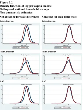
Gasparini and Gluzmann (2009) compute for each country non parametric estimates of the density function of the log per capita income in LCU from both sources of

information. When adjusting incomes for the difference in means, the distributions became reasonably close in most countries. Figure 3.2 shows the comparisons between Gallup and household surveys for the whole region. Both distributions seem to match reasonably well in the case of Latin America, but not in the case of the Caribbean, where the Gallup distribution seems more egalitarian.

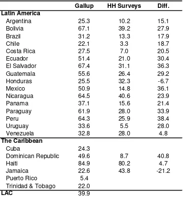
We compute income poverty by applying the international poverty line of US$2 a day adjusted for PPP (Ravallionet al., 1991) to the distributions of household per capita income estimated both from Gallup and national household survey microdata. The US$2-a-day line is a usual standard for international poverty comparisons in the region. Using this line, 39.9% of the population in LAC would be classified as income poor, according to Gallup data. We will use this figure as a benchmark in the following sections of the paper.

Table 3.1 shows the poverty headcount ratios for each country using both sources of information4. On average, poverty in the Gallup Poll is 21 points higher than in national household surveys when using the US$2 line. This gap is naturally linked to the

differences in incomes between the two sources mentioned above. The correlation between poverty estimates using the Gallup survey and those computed with national household survey data is positive and significant. The linear correlation coefficient is 0.62 for LAC, 0.71 for Latin America, and 0.92 without the main income deviants identified above. The Spearman rank correlation coefficient is 0.93. Puerto Rico, Trinidad & Tobago, the Southern Cone and Costa Rica have economies with relatively low income poverty levels, while some Andean and Central American countries are in the other extreme of the ranking. Haiti stands up as the country with the highest incidence of poverty in the region.

In summary, despite a much rougher approximation to per capita income, the picture of poverty in Latin America and the Caribbean that arises from Gallup data is not very different from the one obtained from the national household surveys. Poverty levels are

3_{See Gasparini and Gluzmann (2009) for details.}

4_{See Gasparini and Gluzmann (2009) for estimates using the US$1 line and other poverty indicators.}

highly correlated across both information sources and the poverty rankings are roughly consistent.

We take advantage of the world coverage of the Gallup Poll and compute poverty at the regional level (see Table 3.2).5Poverty in Latin America is lower than in the Caribbean and South Asia, and higher than in East Asia and Pacific, and Eastern Europe and Central Asia.6Income poverty is almost inexistent in Western Europe and North America when measured with the US$2 line. Insufficient observations preclude us to compute income poverty in Middle East and North Africa, and in South Saharan Africa.

4. Objective non-monetary poverty

In this section we extend the measurement of well-being with the Gallup data to other variables beyond income. In particular, we focus the analysis on household

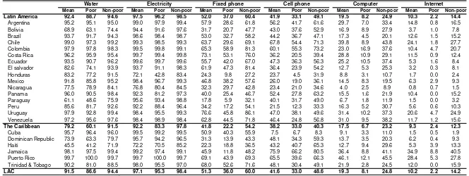
consumption of some services and durable goods. The Gallup Poll 2006 has information on access to a set of basic services–water and electricity -, and communication and information goods and services -phone (fixed and cellular), computer and Internet.7 Table 4.1 shows basic descriptive statistics on those variables by income poverty group based on the US$ 2-a-day line. The first important result is that there is a systematic difference in favor of Latin America, as compared to the Caribben, in terms of access to services and durable goods.

Also, there are significant differences across income poverty groups. In the case of water, 86.6% of the income poor and 94.4% of the income non-poor report having access to water in their dwellings or lots.8The differences are smaller in the case of electricity: the share of respondents with access is 95.3% among the poor and 98.4% among the non-poor.

On average 36% of the income poor in LAC have access to a fixed phone. The share of those with a cell phone is similar (33%). There are substantial differences across countries: while 54.4% of the income poor in Chile have a cell phone, that proportion drops to just 4.5% among the income poor in Honduras. In LAC while 24.8% of the non-poor have a personal computer, the proportion drops to 8.1% for the poor. While

5_{For these comparisons we estimate incomes based on midpoints of brackets in PPP US$ provided by}

Gallup, since we do not have access to incomes in LCU for the rest of the world. For that reason estimates in Tables 3.1 and 3.2 differ.

6_{Chen and Ravallion (2008) find that poverty in LAC is higher than in Eastern Europe & Central Asia}

but lower than in East Asia & Pacific. Sala-i-Martin (2006) reports a ranking similar to that obtained with Gallup data.

7_{Unfortunately, other interesting goods and services are excluded from the analysis because of missing}

information for some countries. For example, data on housing ownership and access to sanitation is only available for Honduras and Nicaragua, while information on access to a television set is not recorded in the surveys of Brazil, Mexico, and Venezuela.

8_{Naturally, propositions like this one are conditional on the methodology adopted to define the income}

10% of LAC respondents have access to Internet in their homes, the share is just 2.2% for the income poor.

Index of non-monetary welfare and poverty

There is a large literature on the measurement of multidimensional poverty

(Bourguignon, 2003; Bourguignon and Chakravarty, 2003; Ducloset al., 2006; Silber, 2007, among others). The key steps are (i) to define the set of variables to be included in the indicator, (ii) to define a structure of weights, and (iii) to set a poverty line.

Regarding the first point, in this section we follow a restricted approach and include the set of goods and services available in the Gallup Poll 2006 listed above: water,

electricity, phone (fixed and mobile), computer and Internet.

To deal with the second step we apply conventional factor analysis methods that take the correlation structure of the chosen variables into account, and, in a way,

endogeneizes the structure of weights.9Thefactorsthat summarize the information contained in the data are obtained by principal component analysis. This method reduces the dimensionality of the problem to a single indicator that allows dividing the population unambiguously into two groups provided a threshold value is set.

This is precisely the third stage. Unfortunately, as in any poverty analysis, the choice of a threshold is highly arbitrary. For comparison with the income poverty approach of the previous section, we set a poverty line in the space of the linear indicator discussed above that implies a share of the LAC population below that threshold equal to the income poverty headcount ratio with the US$ 2 line;i.e. 39.9%. Naturally, imposing this threshold implies losing the possibility of comparing aggregate LAC poverty figures across methodologies (which is anyway a debatable goal), but we gain in comparability at the country level.

It is important to briefly discuss conceptually the approach outlined above. It is

debatable whether this approach really identifies deprivation in a meaningful way. After all, the set of variables used in step (i) includes some goods which are not really basic needs (e.g. computer), and leaves out others which they arguably are (e.g. food). Moreover, as explained above, the “povertyline” has nothing to do with any real

threshold in needs or capacities. What the approach does is to identify relative

deprivation in terms of an index based on the consumption and access to some durable goods and services available in the Gallup survey. That index could be interpreted as a non-monetary proxy for individual well-being. People with less access to water, electricity, phone, computer and Internet presumably have command over a smaller set of all goods and services available in the economy than the rest of the population, and hence they would have higher chances of attaining lower levels of well-being. They are

“deprived”, at least in a relative sense. This limited asset-based approach is an

alternative to the income-based approach implemented in the previous section, where individual well-being is proxied by just the household income per capita.10

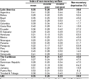
Following this approach we compute a one-dimensional index based on the access to water, electricity, telephone, cell phone, personal computer, and Internet in the 2006 Gallup Poll.11The first three columns of Table 4.2 present mean values of the index–

normalized to a [0, 1] scale- by country and by income poverty group. Last column of Table 4.2 shows the headcount ratios based on the index when setting the threshold to generate an aggregate poverty level of 39.9% (the LAC income poverty rate).

Headcount ratios based on this criterion range from 8.2% in Puerto Rico to 67% in Nicaragua. Southern Cone countries, Costa Rica, Jamaica and Colombia have relatively low levels of objective non-monetary poverty. In the other extreme Nicaragua, Haiti, Paraguay and Honduras rank high in that poverty ladder. When compared to the rest of the world, Latin America looks much better than Sub-Saharan Africa and South Asia (see Table 4.3), and much worse than North America and Western Europe.

5. Subjective poverty

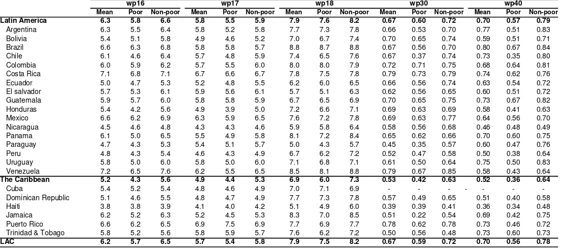
In this section we turn to the analysis of self-assessed welfare based on questions available in the 2006 Gallup data set. Questionswp16,wp17andwp18ask individuals

to rank themselves (“subjectively”) in a 0 to 10 scale, 0 being the worst and 10 the best

present (wp16), past (wp17) and future (wp18) level of welfare. Questionwp30asks whether they are satisfied with their living standard, and questionwp40asks whether in the last year they felt they lacked enough money to satisfy their food needs.12The subjective nature of the answers of these questions is not straightforward, but in all cases questions refer toindividuals’perceptions on how they felt or how much they needed.13

Table 5.1 presents basic descriptive statistics on these variables by income poverty group. First, there is a systematic difference in favor of Latin America, as compared to the Caribbean: all measures are higher for the former group of countries. Perceptions regarding present life are usually less optimistic than those concerning the past (questionswp16andwp17), but the difference is small. The top of the ranking is

occupied by Costa Rica, Venezuela and Puerto Rico, and the bottom by Nicaragua, Peru

10_{This multidimensional approach will be extended to consider other variables in Section 5.}

Unfortunately, a basic needs approach (NBI) similar to that carried out by some LAC statistical offices cannot be implemented with the Gallup 2006, since information is lacking on almost all relevant variables: housing, sanitation and education.

11_{The 2007 Gallup Poll has information on additional variables: automobile, cable TV, DVD player,}

washing machine, and freezer. We computed another one-dimensional index based on these goods plus the set available in the Gallup 2006. Results are available upon request.

12_{Questionswp30andwp40are binary and are recoded so as “1” means satisfied and “0”not-satisfied.} 13_{There are other interesting questions such aswp43(whether in the last year they felt they lacked}

and Haiti. Perceptions regarding the future differ rather dramatically in some countries, as for the case of Brazil, Colombia, Panama, Venezuela, and Jamaica who rank at the top. It is interesting to remark the cases of Argentina and Chile, countries that in spite of performing close to the averages in all other variables, they ranked at the top regarding satisfaction with food needs. Venezuela is another case worth highlighting since exactly the opposite occurs: even tough it is at the top on most measures, it ranks at the bottom in terms of satisfaction with food access. The case of Haiti deserves to be stressed: it ranks at the very bottom ofalldimensions, reflecting the deeply rooted problems this country faces in terms of deprivation.

Regarding responses by income deprivation status, the non-poor, on average, declare to be more satisfied as compared to the poor. However, an interesting result is that when asked about their pasts, the poor and the non-poor provide similar answers.

Index of subjective welfare and poverty

As discussed previously in Section 4, the methodological concerns that arise when translating income into poverty hold alike when trying to classify individuals as into

“deprived/non-deprived”status based on other objective or subjective assessments, in

the sense that the transition between these two situations occurs in a discontinuous fashion when using an underlying continuous welfare measure.

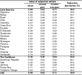
To measure subjective poverty we first construct an index of subjective well-being based on the subjective questions described above. To this end we follow the same methodology as in Section 4, applying a factor analytic approach to this set of variables, and obtaining thefactorsthat summarize the information contained in the data by principal component analysis. Table 5.2 presents results of this aggregation. The top of the ranking based on this index of subjective welfare is occupied by Brazil, Costa Rica, Venezuela and Puerto Rico, and the bottom by Nicaragua, Paraguay and Haiti.

Again, to compute subjective deprivation we set a poverty line in the space of the index of subjective welfare that implies a share of the LAC population below that threshold equal to 39.9% (the LAC income poverty rate using the US$ 2 line). The last column in Table 5.2 shows the results. For example, this implies that in a highly ranked country like Brazil, 28.1% of the households are subjectively deprived. On the other extreme, this figure reaches a dramatic 93.5% for the case of Haiti.

The relatively mild, tough systematic, differences between the responses of the (income based) poor and the non-poor hint towards the true multidimensional nature of welfare: even tough countries differ systematically along subjective welfare, the relationship of this dimension is weak with respect to income, which suggest the inability of income to capture this otherwise relevant welfare dimension. The analysis of these discrepancies is the subject of the next section.

developed regions (Western Europe and North America), but much better than all the other regions. In particular, the differences with regions like Sub-Saharan Africa or Eastern Europe and Central Asia are dramatic.

6. The dimensionality of deprivation

The previous sections dealt with deprivation, understood as low levels of a pre-specified quantifiable notion of welfare: income in Section 3, an index of consumption of durable goods and some services in Section 4, and an index of subjective welfare in Section 5. The underlying method in all sections is the following: a relevant welfare notion is identified, variables in the survey are associated to a particular notion, and then a statistical method is used to produce an index which is later used to classify individuals

into the “poor / non-poor” status.

At this point, a natural question is which is the dimensionality of welfare and hence of deprivation.Even though there is not a clear definition of “dimension” that can be used

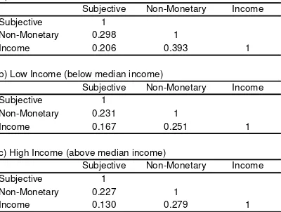
in the study of welfare, the issue refers to the degree of complexity in characterizing an underlying object, close to the mathematical notion of dimension as the number of coordinates needed to specify a point correctly in a given space. In an extreme case there is a single underlying notion of welfare, and from this point of view all questions related to welfare are seen as proxies that differ among themselves due the degree of inaccuracy with respect to the unobserved, single-dimensional welfare concept. In the opposite extreme case, welfare is a truly multidimensional concept that cannot be appropriately captured by any single notion. Hence, from this point of view, questions related to welfare may be summarizing a particular dimension or several of them. As a first approach, Table 6.1 presents correlations among the summary welfare indicators from Sections 3, 4 and 5. That is, we look at household per capita income, and the standardized indices of objective non-monetary and subjective welfare. Correlations are significantly different from zero. The correlation between income and the index of non-monetary welfare is 0.393. The lowest correlation is between

subjective welfare and income (0.206). These results are consistent with previous literature, in the sense that subjective notions of welfare are statistically correlated with income, even though this correlation is low (see, for example Ravallion and Lokshin (2001)). The significant correlation discards the sometimes claimed idea that subjective welfare measures highly idiosyncratic factors that do not obey systematic patterns. Nevertheless, the low correlation suggests that income per-se cannot give account of a considerable part of the variation in welfare.

groups. Interestingly, the correlation between non-monetary welfare and income is higher for richer individuals, while the opposite holds for the correlation between income and subjective welfare.

As a second step, we adopt amore “agnostic” approach and explore directly the

problem of dimensionality of welfare, looking at all the variables considered in Sections 3, 4 and 5, but without clustering them into groups, with the goal of asking how many relevant underlying dimensions of welfare they represent.14

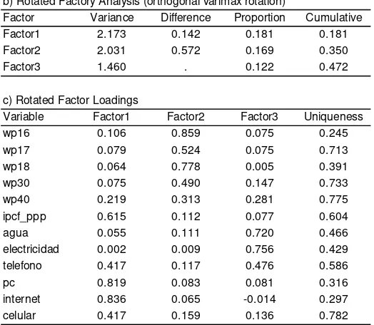
To this end, we follow, again, a factor analytic approach. We apply a principal component factorization for all the countries in LAC. Results are shown in Table 6.2. The first panel of the table presents the eigenvalues associated to each factor, sorted by size, their incremental differences, the proportion associated to each factor and the cumulative proportion of the total variability.

Using the standard rule of retaining factors associated to eigenvlaues greater than one, the method suggests that the 12 variables can be appropriately summarized by three orthogonal factors, the three factors accounting for 0.458 of the total variability. A fourth factor may add to the explanation, nevertheless, we retain three of them, which simplifies interpretation with a minimal loss in explanatory power. It is well known that

factor estimates (“loadings”) are unique up to orthogonal transformations, and hence it

is standard practice to use particular rotations that help interpret the obtained factors. We have used a standard varimax rotation of the three retained factors, and results are shown in the bottom panels of Table 6.2. Each coefficient represents how each variable is weighted in each factor and hence higher values represent variables relatively more important in the factor.

Factor interpretation is usually idiosyncratic, but the results obtained from the rotated coefficients suggest clear patterns. The first factor relies on income, and assets that bear a strong relation with it, like having a computer, access to Internet, or a regular or mobile phone. This is the factor that best represents all the variables. The second factor focuses on the subjective questions, that is, variables weakly correlated with income that still retain relevant information regarding welfare that cannot be accounted by income. Finally, the last factor seems to capture very basic needs, related to having access to water or electricity.

The exploratory analysis derived from a simple factor analytic model suggests that welfare can be appropriately summarized by three orthogonal dimensions. Strikingly, the first one is precisely captured by income and variables strongly related to it. This is an interesting result since it speaks about the importance of income-based assessments of welfare status. Nevertheless, the relevance of the two other factors also shows that welfare is a truly multidimensional phenomenon that cannot be fully captured by income solely. The second factor can belabeled as the “subjective factor”. The fact that

14_{The variables included in the analysis are: per capita income (in PPP USD), access to water, electricity,}

all subjective variables are strongly related among themselves and that they load similarly on the same factor suggests that some average of them may well represent this dimension of welfare. Finally, thethird factor can be labeled as “basic needs”,

suggesting that notions of welfare arising from standard “unsatisfied basic needs”

methods, that include the access to basic services like water or electricity, add relevant information not captured by income.

7. The adequacy of income based poverty lines: implicit poverty

lines

An important result of the previous section is that even in a markedly multidimensional context, income still plays an important role in the characterization of welfare, and in turn, of poverty. Poverty lines are absolute levels that separate the poor from the non-poor, andare usually constructed by “inverting” expenditure patterns, that is, a

consumption basket is exogenously determined, and individuals who cannot afford this basket are rendered as poor. If the relationship between expenditures and income is tight enough, then poverty classifications based on income and expenditures should not differ considerably. On the other hand, self-produced “subjective” classifications arise

from individuals perceptions on their welfare and maybe of others in a reference group,

it is not necessarily an “absolute” notion. In light of the relevance of both income and

subjective based dimensions of welfare, a goal of this section is to assess the

performance of standard income based poverty lines in capturing other dimensions of welfare and hence poverty, in particular the subjective dimension.

We implement a simple exercisethat “inverts”subjective welfare levels in order to find income thresholds that can be used to separate the poor from the non-poor, in a similar fashion to what is currently implemented with expenditures (see Pradhan and Ravallion (2000) for a related approach). Consider a simple example where individuals are asked whether they are“satisfied or dissatisfied with your standard of living”. The goal of the

exercise is to find the income level that best separates the “non-satisfied” from the

“satisfied”: this will be our implicit poverty line.

More concretely, letpbe the probability that an individual classifies herself as

“satisfied” given her level of incomey, and assume that these magnitudes are linked

through a simple possibly non-linear relationp=G( y), whereG( )is an unknown invertible function.

The implicit poverty line is the income level that makes an individual indifferent

between classifying herself as “satisfied” and “non-satisfied”. Suppose that individuals

classify themselves as satisfied if given their income,p>p*, wherep* is a probability threshold that distinguishes the satisfied from the non-satisfied. Then, the implicit poverty lineypis the level of income that solvesyp= G-1(p*).

In order to implement this exercise we need to specify an observable binary variables

is a Bernoulli variable,E(s)=p=G(y). Then, the unknownG(y)function can be estimated through a non-parametric regression estimator. It is tempting at this point to specify a standard parametric form, like a logit or probit, but it seems natural and safer to let the data reveal the form ofG(y)instead of adopting a simple, though possibly unrealistic functional form. For the estimation we apply a standard lowess non-parametric estimator.15

To implement this framework we take questionswp30(satisfaction with living

standard) andwp40(having enough money to buy food), whileyis household per capita income (in PPP US$). Based on this information, the correspondingG(y)functions are estimated non-parametrically.

The choice of the cutoff point is surely arbitrary. A natural choice is to adopt the standard practice of fixing it to the proportion of cases for which the binary indicator is equal to 1 (proportion of satisfied individuals), labeled in the literature as the “base

rate”. Thisis a common practice in probit/logit analysis and has been suggested by

several authors as a “fair” choice (see Menard (2000) for a lengthy discussion on

prediction and classification in binary choice models). It is also common to use 0.5 as a cutoff, that is,predict that an individual is “satisfied” if the predicted probability of

satisfied is greater than that of not-being satisfied. A problem with this second choice is that in the case of questionwp30it implies an out-of-range prediction. More precisely, in the case of food satisfaction (wp40) the proportion of satisfied individuals among those with zero income is 0.41, while the proportion corresponding to those satisfied in general terms (wp30) among the zero income group is 0.59. These figures can be taken as raw estimates of the intercepts of the probability functionsG( ), and then 0.41 and 0.59 are the minimum values of probabilities of satisfaction where each model implicitly operates.

Results are detailed in Table 7.1. The implicit income poverty line for food satisfaction is U$S 36.95 when the probability cutoff is 0.5, and US$ 163.08 when the cutoff is set at 0.659 (the unconditional proportion of satisfied individuals). A comparable figure for overall satisfaction (wp30) is US$ 177.38.

It is interesting to notice that the widely-used US$1-a-day line is equivalent to a monthly income of US$ 32.716. That figure is very close to our estimate of the implicit poverty line associated to the question on food satisfaction withp*=.5 (i.e. monthly US$37). From this analysis the US$1-a-day threshold would be a reasonable poverty line to measure and analyze food deprivation. Instead, the other two implicit lines of Table 7.1 are close to US$5 a day,i.e. values much higher than the typical US$ 2 line used to analyze moderate poverty.

15

Lowess (also known as “loess”) is a robustified local polynomial regression. Basically, an initial local polynomial non-parametric regression is fit using standard k-nearest neighborhood methods, and then it is iteratively robustified (in the sense of making it resistant to outliers) by reweighing observations. See Cleveland (1993) for an intuitive expositions, or Hardle (1990, pp. 192-1993) for a description of the algorithm.

8. Poverty profiles and perceptions

In this section we look at some basic socio-demographic characteristics of the poor, using the three alternative definitions of poverty studied in Sections 3, 4, and 5. Table 8.1 presents an unconditional profile of the poor for the LAC region. We start by splitting the population in age groups and count the proportion of poor in each sub-group. A first relevant result is that age profiles for both income and objective non-monetary poverty exhibit inverse U-shape patterns. The group of young adults -between 26 to 40 years old- presents the highest poverty headcount ratios while 41 to 64 year-olds exhibit the lowest poverty incidence. On the other hand, poverty is strictly increasing when the subjective dimensions are considered. This reversion is an important result for the long-standing debate on the measurement of old age poverty, which bears relevant implications on the targeting of social policies17. In line with these results, income and objective non-monetary poor are on average slightly younger than the non-poor, but the subjectively poor are much older than the subjectively non-poor. Regarding gender, based on the income poverty measure, 46% of the poor are male, compared to 50% of the non-poor. This poverty bias against females is in part due to a higher share of female-headed households among the poor. If the mother lives with their children, and the father lives alone, it is more likely for the mother to be income poor, at least when measuring poverty with per capita income. In terms of household

composition, family sizes are larger among the income poor, and this difference becomes much smaller when the non-monetary and subjective poverty dimensions are considered. Regarding children under 12, the poor differ significantly from the non-poor, based on income poverty: the poor have on average 2.06 children, almost twice the average of the non-poor (1.13). Similar differences, once again, are milder when comparing poor vs. non-poor along the other dimensions. This result is, again,

important for social policy debates, since, it implies that means-tested targeting schemes based on household per capita income, or directly the number of children, may imply significant biases when other dimensions of deprivation are considered. Concerning employment status, only 38% of the income poor in LAC is employed compared to 52% of the non-poor. Again, the gap is narrower when considering the other dimensions. Summarizing, income poverty seems to be more clearly related to socioeconomic characteristics, that is, the income poor and non-poor differ more significantly than when compared along other notions of deprivation. Nevertheless, poverty profiles have several elements in common along the different deprivation dimensions.

Besides socio-demographic characteristics, it is interesting to explore the way individual opinions vary across poverty groups. The Gallup World Poll is rich in providing

information on individuals’opinions on topics such as economic conditions,

government performance and public policies. We are particularly interested in assessing

17_{See Deaton and Paxson (1998), and Gasparini}

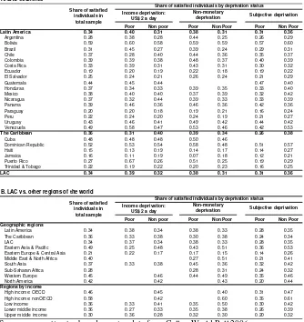
whether opinions about social policies differ or not by poverty status. We concentrate on the question on satisfaction with efforts to deal with the poor (wp131). Table 8.2 presents country means by deprivation status defined using the three dimensions studied in Sections 3, 4, and 5. Panel B in the table presents the results for other regions of world18.

Approximately one third of respondents in LAC countries are satisfied with efforts to deal with the poor. Some cases are interesting to highlight. The top rates of approval to social policy are in the paradigmatic cases of leftist-populist governments (Cuba, Bolivia, and Venezuela). It is naturally impossible to disentangle from the survey whether that result is driven by a more effective social policy in these countries, or by propaganda. In any case, the results suggests that the other LAC countries would have to make more efforts either to turn the social policy more effective, or to show the results better to their people.

Another interesting result is that opinions differ considerably according to poverty status. When defining poverty by income or access to goods and services, poor people are on average more satisfied than the non-poor with social policy. This could be caused by governments doing good things for the poor, who, as direct beneficiaries, can have a better assessment of this help than the non-poor. Alternatively, the non-poor could be better informed on public policies, and therefore can have a better knowledge on the weakness and failures of the social protection system. Disentangling the reason behind this result is beyond the scope of this paper, but it is a priority in our research agenda. When considering the subjective definition of poverty the results change: the poor are less satisfied with efforts to deal with poverty. This reversion could be driven in part by unobservable personality traits: those who are more likely to rank themselves as poor (even when they are not based on objective measures) are also more likely to be less satisfied with a range of other things, including efforts to deal with poverty. The result is challenging: should we partially disregard the low levels of approval of the

subjective-poor since they are in part driven by unobservable individual factors

(pessimism?) that lead some of these people to incorrectly consider themselves as poor? Or should we give special attention to this negative view of the social policy, since the subjective-poor are the real poor who our weak scheme to measure poverty with incomes and consumption of a few goods cannot properly identify?

Compared to other regions of the world, LAC presents lower levels of satisfaction, with the exception of Sub-Saharan Africa and Eastern Europe. The result of higher rates of approval of social policy among the income and the non-monetary poor is also true for some regions but not for all: an exception is the Caribbean. However, along all the regions the subjective poor are less satisfied with social policies that the subjective non-poor.

18_{Notice that means for LAC differ between panels A and B when dividing the population by income}

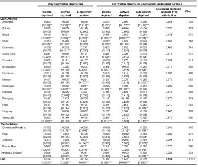
It is possible that perceptions differ between poor and non-poor because of the deprivation status itself, or because of other characteristics that vary between the two groups. To explore this possibility we perform a conditional analysis of responses on the satisfaction with policy efforts to deal with the poor. Probit models of the

probability of being satisfied are estimated for each LAC country using two alternative specifications. The first model includes the three poverty dimensions (income, non-monetary, and subjective), while the second model adds demographic (age, gender) and geographic (urban-rural) controls.19Results are reported in table 8.11.

Estimation results are shown in Table 8.3. They indicate that even when controlling for other poverty measures, and demographic and geographic factors, subjectively poor individuals are more prone than the non-poor to be unsatisfied with efforts to deal with the poor. Other results not shown in the table are that satisfaction with social policies is increasing in age, and it is lower in urban areas, even when controlling for other factors. Besides, in almost all countries, and hence in the region as a whole, the rate of approval to social polices does not significantly vary with gender, even in a conditional model. Finally, we perform microsimulations to address the question of how satisfied on average would people in LAC be, if satisfaction with policies to deal with the poor were driven by the estimated model (the second one) for each country. Alternatively, the same microsimulations inform the satisfaction in each country if the observable characteristics (gender, age, area, besides the three measures of poverty) were those of LAC, and not the real ones of each country. Results from this exercise are shown in the last but one column of Table 8.3. In general, mean predicted probabilities are similar to unconditional proportions from Table 8.2–linear and rank correlation coefficients across countries are 0.94 and 0.91 respectively-, suggesting that what matters the most in determining the degree of satisfaction in a given country is the way perceptions are formed, and not the population characteristics.

9. Concluding remarks

This paper provides evidence on the multiple dimensions of poverty in Latin America and the Caribbean exploiting the Gallup World Poll 2006. In particular, we estimate levels and patterns of income, non-monetary, and subjective poverty for all countries in the region based on Gallup microdata. Since the Gallup Poll has the same questionnaire in all the countries in the world, it provides a unique opportunity to carry out a truly international analysis of social issues.

On average, income poverty in the Gallup Poll is higher than in national household surveys. However, the poverty ranking that arises from the two alternative data sources turns out to be similar. We extend the measurement of well being with the Gallup data to other variables beyond income. In particular, we focus the analysis in household consumption of some services and durable goods. To reduce the dimensionality of the

problem to a single indicator we apply conventional factor analysis methods. The Gallup survey opens a relevant possibility to explore the issues of subjective welfare and deprivation in detail. We find that the rank correlation between income and subjective poverty is positive and significant, suggesting that subjective-based poverty is significantly related to its objective counterpart. On the other hand, the correlation is far from high, suggesting that income represents only part of a more complex,

multidimensional structure behind welfare.

The exploratory analysis derived from a simple factor analytic model suggests that welfare can be appropriately summarized by three dimensions. Strikingly, the first one is precisely captured by income, the second one by an average of the subjective welfare measures, and the third one by variables associated to “basic needs” (water, electricity).

This is an interesting result since, on the one hand, it speaks about the importance of income-based assessments of welfare status, and, on the other hand, shows that welfare is a truly multidimensional phenomenon that cannot be fully captured by income. In order to assess the adequacy of international income-based poverty lines, we implement a simple exercise by inverting subjective welfare levels in order to find income thresholds that can be used to separate the poor from the non-poor. From this analysis the US$1-a-day international line appears to be a reasonable cut-off value to measure and analyze food deprivation.

Referencias

Attanasio, O. and Székely, M. (eds.) (2001).Portrait of the poor. An assets-based approach. IADB.

Bourguignon, F.(2003). From income to endowments: the difficult task of expanding the income poverty paradigm. Delta WP 2003-03.

Bourguignon, F. and S. R. Chakravarty (2003). The Measurement of Multidimensional Poverty.Journal of Economic Inequality, vol. 1 (1), pp. 25-49.

Brandolini, A. and D’Alessio, G. (1998). Measuring Well-Being in the Functioning

Space. General Conference of The International Association for Research in Income and Wealth, Cracow, Poland.

Chen, S. and Ravallion, M. (2007). Absolute poverty measures for the developing world, 1981-2004.PNAS104 (43), 16757-16762.

Chen, S. and Ravallion, M. (2008). "The developing world is poorer than we thought, but no less successful in the fight against poverty," Policy Research Working Paper Series 4703, The World Bank

Cleveland, W. (1993).Visualizing Data, Hobart Press, New Jersey.

Deaton, A. (2007). Income, aging, health and wellbeing around the world: Evidence from the Gallup World Poll. Princeton University, mimeo.

Deaton, A. and Paxson, C. (1998). Poverty among the elderly. In Wise, D. (ed). Inquires in the economic of aging. Chicago University Press for the National Bureau of Economic Research.

Duclos, Jean-Yves, David E. Sahn, Stephen D. Younger (2006). Robust

Multidimensional Poverty Comparisons.The Economic Journal116 (514), 943–

968.

Feres, J. C. and Mancero, X. (2001). Enfoques para la medición de la pobreza. Breve revisión de la literatura. CEPAL, Estudios estadísticos y prospectivos 4.

Gasparini, L. (2003). Different lives: inequality in Latin America and the Caribbean. En Inequality in Latin America and the Caribbean: breaking with history?, chapter 2, Washington D.C: The World Bank.

Gasparini, L. and P. Glüzmann (2009). "Estimating Income Poverty and Inequality from the Gallup World Poll: The Case of Latin America and the Caribbean".

CEDLAS Working Paper N° 83.

Gasparini, L., Alejo, J., Haimovich, F., Olivieri, S. and Tornarolli, L. (2007). Poverty among the Elderly in Latin America and the Caribbean. Background paper for the World Economic and Social Survey 2007. The World Ageing Situation.

Gasparini, L., W. Sosa Escudero, M. Marchionni and S. Olivieri (2009). “Objective and

Perception. Measuring Quality of Life in Latin America. IADB y Brookings Institution Press.

Härdle, W. (1990).Applied Non-parametric Regression, Cambridge University Press, Cambridge

Hädle, W. and Simar, L., (2003),Applied Multivariate Statistical Analysis, Springer, New York.

Menard, S. (2000). Coefficients of determination for multiple logistic regression analysis,The American Statistician, 54-1, pp. 17-24.

Osberg, L. and Sharpe, A. (2005). How Should We Measure Well-being?.Review of Income and Wealth, 51.

Pradhan, M. and Ravallion, M.(2000). "Measuring Poverty Using Qualitative Perceptions Of Consumption Adequacy,"The Review of Economics and Statistics, MIT Press, vol. 82(3), pages 462-471.

Ravallion, M., Datt, G., and van de Walle, D. (1991). "Quantifying Absolute Poverty in the Developing World,"Review of Income and Wealth, Blackwell Publishing, vol. 37(4), pages 345-61, December.

Ravallion, M. and Lokshin, M. (2002). Self-rated economic welfare in Russia, European Economic Review, 46:1453-1473.

Ravallion, M. and Lokshin, M. (2001). "Identifying Welfare Effects from Subjective Questions,"Economica, London School of Economics and Political Science, vol. 68(271), pages 335-57, August.

Sala-i-Martin, X. (2006). The world distribution of income: falling poverty and

…convergence, period.The Quarterly Journal of EconomicsCXXI (2), May.

Sen, A. (1984). Rights and Capabilities. In A. Sen,Resources, Values and Development. Oxford: Basil Blackwell.

Table 2.1

Number of observations Gallup World Poll 2006

Countries in LAC Observations Regions in the world Observations Latin America 17,144 Geographic regions

Argentina 1,000 LAC 21,200 Bolivia 1,000 East Asia & Pacific 19,630 Brazil 1,029 Estern Europe & Central Asia 32,757 Chile 1,007 Middle East & North Africa 15,837 Colombia 1,000 South Asia 7,380 Costa Rica 1,002 Sub-Saharan Africa 26,506 Ecuador 1,067 Western Europe 16,073 El Salvador 1,000 North America 2,356 Guatemala 1,021

Honduras 1,000 Mexico 1,007 Nicaragua 1,001 Panama 1,005 Paraguay 1,001 Peru 1,000 Uruguay 1,004 Venezuela 1,000

The Caribbean 4,056

Cuba 1,000 Dominican Republic 1,000 Haiti 505 Jamaica 543 Puerto Rico 500 Trinidad & Tobago 508

LAC 21,200

Table 3.1

Poverty in LAC from the Gallup survey and household surveys

Headcount ratio, US$ 2-a-day line

Gallup HH Surveys Diff. Latin America

Argentina 25.3 10.2 15.1 Bolivia 67.1 39.2 27.9 Brazil 31.2 13.3 17.9 Chile 22.1 3.3 18.7 Costa Rica 27.5 7.0 20.5 Ecuador 51.4 21.0 30.4 El Salvador 67.4 31.1 36.3 Guatemala 55.6 26.4 29.2 Honduras 25.5 32.3 -6.7 Mexico 50.9 14.8 36.1 Nicaragua 64.5 40.6 23.9 Panama 37.1 15.6 21.4 Paraguay 61.9 28.0 33.9 Peru 64.3 25.9 38.4 Uruguay 33.6 5.5 28.0 Venezuela 32.8 28.0 4.8

The Caribbean

Cuba 24.3

Dominican Republic 49.6 8.7 40.8 Haiti 84.9 80.2 4.7 Jamaica 22.6 43.8 -21.2 Puerto Rico 5.4

Trinidad & Tobago 22.0

LAC 39.9

Source: own estimates based on microdata from Gallup World Poll 2006 and national household surveys.

Table 3.2

Poverty in the regions of the world Headcount ratio, US$2 a day line

Poverty

Latin America 17.6 The Caribbean 23.3

LAC 18.0

East Asia & Pacific 13.3 Estern Europe & Central Asia 10.2 South Asia 23.5 Western Europe 0.0 North America 0.0

22

Table 4.1

Some services and durable goods. Basic descriptive statistics. Gallup survey 2006

Mean Poor Non-poor Mean Poor Non-poor Mean Poor Non-poor Mean Poor Non-poor Mean Poor Non-poor Mean Poor Non-poor

Latin America 92.4 88.7 94.6 97.5 96.2 98.5 52.0 37.0 60.4 41.9 33.1 49.1 19.5 8.2 24.9 10.3 2.2 14.4

Argentina 95.2 95.1 95.0 99.0 97.9 99.4 57.9 28.6 61.8 56.2 41.7 61.6 29.7 7.0 33.4 14.8 0.8 16.5

Bolivia 68.9 63.1 74.4 94.4 91.6 97.6 31.7 20.7 47.7 43.0 37.6 52.9 16.9 8.9 27.9 3.7 1.0 7.8

Brazil 93.7 91.7 94.3 98.6 98.4 98.7 53.0 32.7 58.2 44.2 36.7 47.1 17.3 4.5 20.1 12.6 1.5 15.2

Chile 99.0 97.3 99.2 99.3 98.5 99.3 63.7 29.6 69.1 67.8 54.4 71.3 39.8 8.9 43.8 24.1 1.8 27.7

Colombia 97.9 97.8 98.3 99.5 99.8 99.1 65.3 58.9 81.3 60.1 55.3 73.2 23.0 16.9 37.6 10.4 4.7 20.7

Costa Rica 96.2 95.9 95.4 99.7 99.4 99.8 73.1 53.1 76.0 36.2 20.5 39.4 28.8 10.9 29.1 11.5 0.9 12.4

Ecuador 93.5 90.7 96.2 99.6 99.7 99.6 55.7 42.0 67.0 47.3 36.3 56.3 25.2 10.5 37.4 5.3 1.6 8.4

El salvador 82.6 74.1 93.9 93.7 91.1 98.3 61.9 47.3 81.4 36.4 23.9 54.2 12.7 5.3 25.3 3.2 0.3 8.1

Honduras 83.2 77.2 91.5 72.1 42.8 83.4 24.3 9.8 27.2 23.7 4.5 31.9 8.8 3.1 10.7 1.7 0.0 2.4

Mexico 91.8 85.8 95.2 98.4 96.7 99.3 46.8 38.2 57.6 26.0 19.0 36.1 14.5 8.3 19.5 6.3 2.9 9.3

Nicaragua 77.5 78.9 84.1 76.8 80.4 84.5 32.3 29.7 42.8 23.4 21.0 34.6 4.0 2.5 8.9 0.8 0.7 1.5

Panama 96.0 90.5 98.4 92.3 81.2 97.3 40.0 25.4 46.7 52.4 27.8 63.2 15.5 1.6 21.9 10.4 0.0 15.2

Paraguay 61.1 48.6 75.9 95.6 93.4 98.8 17.8 5.9 32.1 40.1 31.7 49.0 6.7 1.8 11.9 1.5 0.0 3.2

Peru 85.6 81.7 92.6 92.2 88.4 96.4 34.2 17.2 54.1 21.5 12.3 33.3 16.3 5.2 30.7 5.6 0.6 10.3

Uruguay 97.9 92.8 99.4 98.4 95.5 99.3 76.6 45.8 86.1 47.0 38.1 49.6 31.4 10.2 37.3 20.6 4.7 24.9

Venezuela 97.2 95.6 97.6 98.4 98.9 98.4 62.8 44.5 71.8 46.4 24.8 56.8 31.0 9.5 38.2 11.7 1.2 15.6

The Caribbean 79.2 60.1 91.5 92.2 83.3 97.8 41.8 22.2 54.2 38.2 33.0 40.3 17.5 6.7 23.2 9.3 2.4 12.3

Cuba 95.7 96.4 96.0 99.5 99.2 99.5 50.9 40.3 55.9 7.5 6.7 8.3 9.1 3.3 11.0 1.5 0.5 1.9

Dominican Republic 73.9 63.3 79.7 95.7 94.2 96.5 31.3 13.9 43.3 48.1 34.3 59.3 13.7 3.5 20.3 6.2 0.4 9.3

Haiti 45.5 41.2 71.9 72.2 70.5 85.2 22.3 18.8 36.5 43.2 40.7 65.3 12.7 9.4 29.6 5.3 3.9 13.3

Jamaica 98.1 97.5 99.4 99.2 97.4 99.1 45.9 11.8 48.2 75.9 66.2 80.5 36.4 8.8 41.1 34.9 8.8 40.5

Puerto Rico 99.7 100.0 99.7 99.7 100.0 99.7 69.1 43.9 69.3 65.5 39.6 66.3 46.1 12.1 45.5 28.4 5.3 27.8

Trinidad & Tobago 90.2 81.0 88.5 98.0 95.5 97.0 68.0 52.6 71.6 48.1 30.4 49.1 21.9 2.8 24.5 12.0 0.0 15.9

LAC 91.5 86.6 94.4 97.1 95.3 98.4 51.3 36.0 60.0 41.6 33.0 48.6 19.3 8.1 24.8 10.2 2.2 14.2

Computer Internet

Water Electricity Fixed phone Cell phone

Table 4.2

Objective non-monetary welfare and poverty in LAC Gallup survey 2006

mean income

poor

income non-poor

Latin America 0.35 0.26 0.39 39.6

Argentina 0.41 0.26 0.44 19.4

Bolivia 0.28 0.22 0.35 52.6

Brazil 0.35 0.25 0.38 45.6

Chile 0.49 0.28 0.53 11.7

Colombia 0.39 0.34 0.49 17.7

Costa Rica 0.40 0.28 0.41 19.8

Ecuador 0.36 0.28 0.42 27.2

El Salvador 0.29 0.23 0.39 37.6

Honduras 0.21 0.13 0.25 63.5

Mexico 0.30 0.25 0.35 45.8

Nicaragua 0.20 0.20 0.25 67.0

Panama 0.33 0.20 0.38 31.7

Paraguay 0.22 0.17 0.27 63.8

Peru 0.28 0.20 0.38 56.9

Uruguay 0.45 0.28 0.50 14.6

Venezuela 0.41 0.28 0.46 32.5

The Caribbean 0.31 0.21 0.37 43.6

Cuba 0.27 0.24 0.28 47.5

Dominican Republic 0.28 0.20 0.34 47.0

Haiti 0.22 0.19 0.36 64.2

Jamaica 0.51 0.29 0.55 15.8

Puerto Rico 0.53 0.31 0.53 8.2

Trinidad & Tobago 0.38 0.24 0.40 21.9

LAC 0.35 0.26 0.39 39.9

Index of non-monetary welfare _Non-monetary

deprivation (%)

Source: own estimates based on microdata from Gallup World Poll 2006.

Note: the index is based on access to water, electricity, telephone, personal computer, Internet and cell phone. Poverty line set to generate a LAC headcount ratio similar to the LAC income poverty ratio with the US$ 2-a-day line (39.9%).

Table 4.3

Objective non-monetary welfare and poverty in other regions of the world. Gallup survey 2006

mean income

poor

income non-poor Geographic Regions

Latin America & The Caribbean 0.39 0.28 0.41 18.0

Eastern Asia & Pacific 0.36 0.20 0.38 52.4

Eastern Europe & Central Asia 0.44 0.25 0.45 33.8

Middle East & North Africa 0.55 25.1

South Asia 0.16 0.09 0.18 89.4

Sub-Saharan Africa 0.11 92.3

Western Europe 0.81 0.80 1.0

North America 0.88 0.88 0.0

Regions by Income

High Income: OECD 0.87 0.87 0.8

High Income: non OECD 0.78 0.77 2.3

Low Income 0.15 0.13 0.22 87.8

Lower Middle Income 0.34 0.22 0.37 50.2

Upper Middle Income 0.43 0.28 0.45 24.4

Index of non-monetary welfare

Non-monetary deprivation (%)

Source: own estimates based on microdata from Gallup World Poll 2006

24

Table 5.1

Questions on subjective welfare. Basic descriptive statistics. Gallup survey 2006

Mean Poor Non-poor Mean Poor Non-poor Mean Poor Non-poor Mean Poor Non-poor Mean Poor Non-poor

Latin America 6.3 5.8 6.6 5.8 5.5 5.9 7.9 7.6 8.2 0.67 0.60 0.72 0.70 0.57 0.79

Argentina 6.3 5.5 6.4 5.8 5.2 5.8 7.7 7.3 7.8 0.66 0.53 0.70 0.77 0.51 0.83

Bolivia 5.4 5.1 5.8 4.9 4.6 5.2 7.0 6.7 7.4 0.70 0.65 0.74 0.59 0.51 0.71

Brazil 6.6 6.3 6.8 5.8 5.8 5.7 8.8 8.7 8.8 0.67 0.56 0.70 0.80 0.67 0.84

Chile 6.1 4.6 6.4 5.7 4.8 5.9 7.4 6.5 7.6 0.67 0.37 0.74 0.73 0.35 0.80

Colombia 6.0 5.9 6.2 5.7 5.5 6.0 8.0 8.0 7.9 0.72 0.71 0.75 0.68 0.64 0.81

Costa Rica 7.1 6.8 7.1 6.7 6.6 6.7 7.8 7.5 7.8 0.79 0.73 0.79 0.74 0.62 0.76

Ecuador 5.0 4.7 5.3 5.2 4.8 5.5 6.2 6.0 6.5 0.66 0.56 0.74 0.63 0.54 0.72

El salvador 5.7 5.3 6.1 5.9 5.6 6.1 5.7 5.1 6.3 0.62 0.56 0.65 0.60 0.51 0.72

Guatemala 5.9 5.7 6.0 5.8 5.8 5.9 6.7 6.5 6.9 0.70 0.65 0.75 0.73 0.67 0.82

Honduras 5.4 4.2 5.6 4.9 3.9 5.0 7.2 6.6 7.1 0.69 0.63 0.69 0.58 0.41 0.63

Mexico 6.6 6.2 6.9 6.3 5.9 6.5 7.6 7.2 7.8 0.69 0.63 0.77 0.64 0.56 0.70

Nicaragua 4.5 4.6 4.8 4.3 4.3 4.6 5.9 5.8 6.4 0.58 0.56 0.68 0.46 0.48 0.49

Panama 6.1 5.0 6.5 5.5 4.9 5.8 8.1 7.2 8.4 0.65 0.62 0.66 0.70 0.60 0.75

Paraguay 4.7 4.3 5.3 5.4 5.1 5.7 5.0 4.3 5.7 0.45 0.35 0.57 0.60 0.47 0.76

Peru 4.8 4.3 5.4 4.6 4.3 4.9 6.7 6.2 7.2 0.52 0.47 0.58 0.50 0.38 0.64

Uruguay 5.8 5.0 6.0 5.8 5.0 6.0 7.1 6.8 7.1 0.61 0.50 0.64 0.75 0.50 0.83

Venezuela 7.2 6.5 7.6 6.2 5.5 6.5 8.5 8.1 8.8 0.79 0.67 0.85 0.58 0.43 0.64

The Caribbean 5.2 4.3 5.6 4.9 4.4 5.3 6.9 6.0 7.3 0.53 0.42 0.63 0.52 0.36 0.64

Cuba 5.4 5.2 5.4 4.8 4.6 4.9 7.0 7.1 6.9 - - -

Dominican Republic 5.1 4.6 5.5 4.8 4.7 4.9 7.7 7.3 7.8 0.57 0.49 0.65 0.51 0.40 0.58

Haiti 3.8 3.8 3.9 4.1 4.0 4.2 5.1 4.9 6.0 0.39 0.39 0.41 0.36 0.34 0.48

Jamaica 6.2 5.2 6.3 5.2 4.5 5.3 8.3 7.0 8.5 0.51 0.22 0.54 0.69 0.42 0.75

Puerto Rico 6.6 6.2 6.5 6.9 7.5 6.9 7.7 6.9 7.7 0.78 0.62 0.78 0.73 0.46 0.72

Trinidad & Tobago 5.8 5.2 5.6 5.8 5.9 5.7 7.6 6.2 7.2 0.50 0.56 0.48 0.73 0.60 0.73

LAC 6.2 5.7 6.5 5.7 5.4 5.8 7.9 7.5 8.2 0.67 0.59 0.72 0.70 0.56 0.78

wp16 wp17 wp18 wp30 wp40

Source: own estimates based on microdata from Gallup World Poll 2006

Note:wp16,wp17, andwp18ask individuals to rank themselves in a 0 to 10 scale, 0 being the worst and 10 the best present (wp16), past (wp17), and future (wp18) possible life;wp30asks individuals whether they are satisfied with their living standard and questionwp40asks whether in the last year they felt they lacked enough money to satisfy

Table 5.2

Subjective welfare and poverty in LAC Gallup survey 2006

mean income

poor

income non-poor

Latin America 0.68 0.63 0.71 38.8

Argentina 0.68 0.59 0.70 39.6

Bolivia 0.60 0.56 0.65 59.7

Brazil 0.72 0.68 0.73 28.1

Chile 0.66 0.49 0.69 44.3

Colombia 0.67 0.66 0.70 40.8

Costa Rica 0.73 0.70 0.74 27.7

Ecuador 0.57 0.53 0.61 64.6

El Salvador 0.58 0.53 0.63 61.9

Guatemala 0.64 0.62 0.66 51.5

Honduras 0.61 0.51 0.61 54.2

Mexico 0.68 0.64 0.72 41.0

Nicaragua 0.51 0.50 0.56 71.9

Panama 0.67 0.59 0.70 40.9

Paraguay 0.50 0.43 0.57 79.2

Peru 0.54 0.49 0.60 67.8

Uruguay 0.64 0.55 0.66 48.9

Venezuela 0.74 0.66 0.77 26.9

The Caribbean 0.56 0.46 0.64 64.8

Dominican Republic 0.59 0.53 0.62 58.1

Haiti 0.42 0.41 0.46 93.5

Jamaica 0.66 0.53 0.68 43.0

Puerto Rico 0.71 0.67 0.71 36.8

Trinidad & Tobago 0.64 0.54 0.62 48.2

LAC 0.68 0.62 0.71 39.9

Index of subjective welfare

Subjective deprivation (%)

Source: own estimates based on microdata from Gallup World Poll 2006.

Note: the index is based on questionswp16, wp17, wp18, wp30,andwp40. Poverty line set to generate a LAC headcount ratio similar to the LAC income poverty ratio with the US$ 2-a-day line (39.9%).

Table 5.3

Subjective welfare and poverty in other regions of the world. Gallup survey 2006

mean income poor

income non-poor

Latin America & The Caribbean 0.67 0.58 0.69 18.0

Eastern Asia & Pacific 0.60 0.45 0.63 24.2 Eastern Europe & Central Asia 0.53 0.47 0.54 41.8 Middle East & North Africa 0.62 25.0 South Asia 0.58 0.49 0.60 31.7 Sub-Saharan Africa 0.47 55.5 Western Europe 0.73 0.72 7.1 North America 0.74 0.73 8.1

Regions by Income

High Income: OECD 0.72 0.72 8.9 High Income: non OECD 0.71 0.67 9.4 Low Income 0.55 0.48 0.60 37.6 Lower Middle Income 0.57 0.50 0.60 32.9 Upper Middle Income 0.62 0.59 0.64 32.9

Index of subjective welfare _Subjective

deprivation (%)

Source: own estimates based on microdata from Gallup World Poll 2006

Table 6.1

Correlations among welfare indicators

a) All Individuals

Subjective Non-Monetary Income

Subjective 1

Non-Monetary 0.298 1

Income 0.206 0.393 1

b) Low Income (below median income)

Subjective Non-Monetary Income

Subjective 1

Non-Monetary 0.231 1

Income 0.167 0.251 1

c) High Income (above median income)

Subjective Non-Monetary Income

Subjective 1

Non-Monetary 0.227 1

Income 0.130 0.279 1

Table 6.2

Factor analysis results

a) Unrotated Factor Analysis

Factor Eigenvalue Difference Proportion Cumulative

Factor1 2.989 1.490 0.249 0.249

Factor2 1.499 0.323 0.125 0.374

Factor3 1.176 0.185 0.098 0.472

Factor4 0.991 0.075 0.083 0.555

Factor5 0.916 0.093 0.076 0.631

Factor6 0.823 0.071 0.069 0.700

Factor7 0.753 0.019 0.063 0.762

Factor8 0.734 0.015 0.061 0.823

Factor9 0.719 0.049 0.060 0.883

Factor10 0.669 0.292 0.056 0.939

Factor11 0.377 0.024 0.031 0.971

Factor12 0.354 . 0.030 1.000

b) Rotated Factory Analysis (orthogonal varimax rotation)

Factor Variance Difference Proportion Cumulative

Factor1 2.173 0.142 0.181 0.181

Factor2 2.031 0.572 0.169 0.350

Factor3 1.460 . 0.122 0.472

c) Rotated Factor Loadings

Variable Factor1 Factor2 Factor3 Uniqueness

wp16 0.106 0.859 0.075 0.245

wp17 0.079 0.524 0.075 0.713

wp18 0.064 0.778 0.005 0.391

wp30 0.075 0.490 0.147 0.733

wp40 0.219 0.313 0.281 0.775

ipcf_ppp 0.615 0.112 0.077 0.604

agua 0.055 0.111 0.720 0.466

electricidad 0.002 0.009 0.756 0.429

telefono 0.417 0.117 0.476 0.586

pc 0.819 0.083 0.081 0.316

internet 0.836 0.065 -0.014 0.297

celular 0.417 0.159 0.136 0.782

Source: own estimates based on microdata from Gallup World Poll 2006.

Table 7.1

Implicit poverty lines

Enough money to buy food

Satisfaction with living standard

mean zero obs 0.41 0.59

p*=0.5 36.95

p*=0.659 163.08

p*=0.637 177.38

Table 8.1

Poverty profiles in LAC

Poor Non-poor Poor Non-poor Poor Non-poor Age group

[16,25] 0.37 0.63 0.40 0.60 0.32 0.68 [26,40] 0.41 0.59 0.42 0.58 0.40 0.60 [41,64] 0.36 0.64 0.38 0.62 0.47 0.53

[65+] 0.39 0.61 0.38 0.62 0.50 0.50

Mean age 36.95 37.42 36.85 37.29 39.07 34.58 Share males 0.46 0.50 0.47 0.49 0.49 0.48 Family size 4.77 3.76 4.30 4.04 4.37 4.03 Children (<12) 2.06 1.13 1.66 1.38 1.67 1.43 Employed 0.38 0.52 0.41 0.46 0.41 0.47 Satisfaction with efforts to deal with the poor 0.39 0.32 0.38 0.31 0.31 0.36

Income Objective non-monetary Subjective

Source: own estimates based on microdata from Gallup World Poll 2006.

Table 8.2

Satisfaction with efforts to deal with the poor by poverty status

A. LAC countries

Poor Non poor Poor Non Poor Poor Non Poor

Latin America 0.34 0.40 0.31 0.38 0.31 0.31 0.36

Argentina 0.28 0.38 0.28 0.44 0.25 0.26 0.29 Bolivia 0.59 0.60 0.58 0.59 0.59 0.57 0.60 Brazil 0.31 0.45 0.27 0.39 0.24 0.29 0.31 Chile 0.37 0.28 0.40 0.44 0.36 0.35 0.37 Colombia 0.39 0.39 0.38 0.48 0.37 0.40 0.39 Costa Rica 0.33 0.39 0.31 0.43 0.31 0.30 0.32 Ecuador 0.19 0.20 0.19 0.22 0.18 0.19 0.22 El Salvador 0.25 0.24 0.21 0.26 0.24 0.21 0.29

Guatemala 0.44 0.45 0.44 0.47 0.40

Honduras 0.37 0.34 0.33 0.39 0.35 0.33 0.40 Mexico 0.38 0.40 0.40 0.37 0.39 0.32 0.42 Nicaragua 0.37 0.32 0.44 0.39 0.33 0.33 0.39 Panama 0.39 0.46 0.36 0.46 0.36 0.42 0.36 Paraguay 0.20 0.20 0.18 0.19 0.21 0.16 0.24 Peru 0.22 0.24 0.20 0.24 0.19 0.21 0.27 Uruguay 0.43 0.46 0.41 0.49 0.42 0.44 0.42 Venezuela 0.49 0.58 0.47 0.53 0.46 0.42 0.53

The Caribbean 0.36 0.31 0.40 0.39 0.34 0.26 0.38

Cuba 0.48 0.48 0.48 0.50 0.46

Dominican Republic 0.52 0.53 0.54 0.58 0.48 0.51 0.57 Haiti 0.15 0.13 0.19 0.14 0.17 0.14 0.27 Jamaica 0.16 0.11 0.19 0.07 0.18 0.12 0.21 Puerto Rico 0.27 0.67 0.26 0.51 0.25 0.19 0.29 Trinidad & Tobago 0.22 0.19 0.22 0.20 0.23 0.16 0.25

LAC 0.34 0.39 0.32 0.38 0.31 0.31 0.36

B. LAC vs. other regions of the world

Poor Non poor Poor Non Poor Poor Non Poor Geographic regions

Latin America 0.34 0.38 0.34 0.38 0.33 0.28 0.35 The Caribbean 0.36 0.33 0.38 0.30 0.38 0.24 0.34

LAC 0.34 0.37 0.34 0.38 0.33 0.28 0.35

Eastern Asia & Pacific 0.49 0.25 0.48 0.43 0.51 0.36 0.53 Eastern Europe & Central Asia 0.21 0.22 0.17 0.17 0.15 0.14 0.26 Middle East & North Africa 0.40 0.27 0.51 0.21 0.41 South Asia 0.37 0.33 0.38 0.45 0.36 0.32 0.42 Sub-Saharan Africa 0.28 0.28 0.31 0.24 0.32 Western Europe 0.45 0.46 0.44 0.49 0.35 0.46

North America 0.42 0.42 0.43 0.20 0.44

Regions by income

High income: OECD 0.46 0.45 0.40 0.31 0.47 High income: nonOECD 0.58 0.42 0.60 0.35 0.61 Low income 0.36 0.33 0.41 0.35 0.50 0.30 0.42 Lower middle income 0.36 0.27 0.33 0.35 0.38 0.26 0.39 Upper middle income 0.30 0.36 0.28 0.32 0.30 0.20 0.32

Share of satisfied individuals in total sample

Income deprivation: US$ 2 a day

Share of satisfied individuals by deprivation status Non-monetary

deprivation Subjective deprivation Share of satisfied

individuals in total sample

Subjective deprivation Share of satisfied individuals by deprivation status

Income deprivation: US$ 2 a day

Non-monetary deprivation

Source: own estimates based on microdata from Gallup World Poll 2006

Panel A Note: Poverty line set to generate a LAC headcount ratio similar to the LAC income poverty ratio with the US$ 2-a-day line (39.9%).