© 2018 Universidad Nacional Autónoma de México, Centro de Ciencias de la Atmósfera. This is an open access article under the CC BY-NC License (http://creativecommons.org/licenses/by-nc/4.0/).
Total ozone mass calculation to assess the global ozone behavior
José Luis PINEDO-VEGA*, Carlos RÍOS-MARTÍNEZ, Mario MOLINA-ALMARAZ, J. Ignacio DÁVILA-RANGEL and Fernando MIRELES-GARCÍA
Universidad Autónoma de Zacatecas, Ciprés 10, Fraccionamiento la Peñuela, 98000 Zacatecas, Zacatecas, México *Corresponding author; email: jlpv85@gmail.com
Received: March 2, 2017; accepted: March 13, 2018
RESUMEN
Utilizando la totalidad de las mediciones de satélite obtenidas diariamente con el espectrómetro para mapear ozono total (TOMS, por sus siglas en inglés) versión 8 y el instrumento para monitoreo del ozono (OMI, por sus siglas en inglés) nivel 3 de la NASA, en este trabajo se presenta la cuantificación de la masa total global y hemisférica de ozono y el análisis de sus variaciones interanuales. El valor promedio global de la masa de ozono entre noviembre de 1978 y noviembre de 1979 fue de 3.1283 ± 0.1337 × 10¹² kg mientras que de noviembre de 2004 a noviembre de 2005 fue de 2.9979 ± 0.0917 × 10¹² kg. La diferencia (1.3033 ± 0.3221 × 10¹¹ kg) representa una disminución de 4.2 ± 0.3% en 26 años (1.615 ± 0.113% por década), alrededor de 3% correspondiente al hemisferio norte y 5% al hemisferio sur, lo cual implica una disminución de 1.2 y 2.0% por década, respectivamente. La diferencia en las tendencias del ozono entre los hemisferios norte y sur evidencia cambios importantes en la distribución geográfica del ozono en el hemisferio sur. El ajuste lineal arroja resultados similares: de noviembre de 1978 a noviembre de 1991 se observa una disminución global de 4.72 × 10⁹ kg por año, lo cual representa una pérdida de 1.5 % por década. Adicionalmente se encontró una variación interanual neta de 16% en la cantidad total de ozono existente durante los equinoccios, periodos en que se alcanza el valor máximo de la masa total de ozono.
ABSTRACT
This work presents an assessment of the global and hemispheric total ozone mass and its interannual vari-ations, using the total number of daily satellite measurements from the Total Ozone Mapping Spectrom-eter (TOMS) version 8 and Ozone Monitoring Instrument (OMI) level 3. The mean total ozone mass was 3.1283 ± 0.1337 × 10¹² kg from November 1978 to November 1979, and 2.9979 ± 0.0917 × 10¹² kg from November 2004 to November 2005. The difference (1.3033 ± 0.3221 × 10¹¹ kg) represents a 4.2 ± 0.3% decrease in 26 yrs (1.615 ± 0.113% per decade), around 3% corresponding to the Northern Hemisphere and 5% corresponding to the Southern Hemisphere; 1.2 and 2.0% per decade, respectively. Differences in total ozone mass trends between Northern and Southern hemispheres indicate a change in geographic ozone distribution in the Southern Hemisphere. A linear fit between November 1978 and November 1991 shows a global ozone decrease of 4.72 × 10⁹ kg per year, representing a loss of 1.5% per decade. Additionally, we found a net interannual variation of 16% of the total quantity existing during the equinoxes, when the maximum annual total ozone mass is reached.
1. Introduction
Ozone trends have been analyzed by diverse methods in many local and regional studies over various time peri-ods. Few studies have moved beyond the total column ozone (TCO) analysis to quantify the total amount of ozone in the atmosphere, and analyzing its seasonal variations and interannual trends. Dave and Mateer (1967) conducted a preliminary study of the feasi-bility of determining total atmospheric ozone from satellite measurements. Bodeker et al. (2001) noted that global ozone mass levels were aproximately 3 × 10¹² kg.
We now present a quantification of the total ozone mass and its global and hemispheric seasonal variations, using the total number of daily measure-ments from the Total Ozone Mapping Spectrome-ter (TOMS) version 8 and the Ozone Monitoring Instrument (OMI) level 3. TOMS and OMI daily measurements yield the TCO daily geographical distribution for all regions except those covered by the polar nights. Therefore, it is possible to analyze trends of total ozone mass by using all of the TCO measurements contained in the daily files, without restricting the analysis to the daily or monthly average values.
First, we analyzed the data integrity of measure-ments different from zero in the daily files of TOMS and OMI, hereafter called recorded measurements. We quantified total ozone mass by integrating all TCO values over the entire Earth’s surface (except the polar regions with low solar illumination), taking into account the geographical location of each parcel measured.
Although there is a relationship between TCO and total ozone mass, it is not linear. Each value of TCO, TOMS and OMI corresponds to a parcel with a defined geographical location. The area of each parcel is a function of the cosine of the latitude. While at the equator each TOMS’ observation parcel has an area of 4327 km2, at latitude 60º each plot has an
area of 2183.5 km2. Thus, the amount of ozone for a
certain TCO value at the equator is twice the amount of ozone at latitude 60º.
There is a substantial difference between TCO measurements and the corresponding total ozone mass. Hence, to evaluate the behavior of global ozone, it is not enough to assess trends in TCO; it is necessary to quantify the total ozone mass over time.
2. Materials and methods
TOMS and OMI are the most prolific generators of daily TCO data in existence. Aboard Nimbus-7, TOMS provided global measurements of TCO from November 1, 1978 to May 6, 1993. Aboard Mete-or-3, TOMS operated from August 22, 1991 until the Meteor-3 failure in November 25, 1994. Earth Probe TOMS was launched on July 2, 1996 and continued coverage until December 14, 2005. The Aura space-craft was launched on July 15th, 2004 with the OMI instruments aboard, and continues to collect data.
All TOMS data files (gathered aboard Nimbus-7, Meteor-3, and Earth Probe) have the same structure: each daily global file covers 288 longitudinal sections (each measuring 1.25º) from 179.375º W to 179.375º E, and 180 meridional sections (each measuring 1.00º) from 89.5º S to 89.5º N. Thus, a daily TOMS file contains data for 51 840 parcels measuring 1º latitude by 1.25º longitude.
OMI data files (gathered onboard the Aura satellite) have a slightly different structure. Coverage consists of 360 longitudinal sections from 179.5º W to 179.5º E and 180 meridional sections from 89.5º S to 89.5º N, each measuring 1º. Thus, each daily OMI file con-tains data for 64 800 parcels measuring 1º latitude × 1º longitude.
However, TOMS and OMI never register a 100% global coverage. Since the TCO measurement prin-ciple depends on the reflection of solar UV radiation in certain spectral bands, parcels in polar night or low-light areas cannot be measured. On solstices (June 21-22 in the Southern Hemisphere; December 21-22 in the Northern Hemisphere) TOMS and OMI fail to cover a significant polar region extending up to 29º latitude. During spring and autumn equinoxes (March 20-21 and September 22-23), the unmeasur-able region shrinks to 6º latitude around the Poles.
Up to about 48 600 daily values of TCO can be measured at the equinox vs. about 43 200 values at the solstice. During equinoxes, TOMS and OMI are able to record most of the ozone present in the atmosphere. The unmeasured ozone at the poorly-lit poles, while important in terms of global ozone transport, is not important from the point of view of ozone produc-tion and destrucproduc-tion; therefore it was not taken into account for the purposes of this study.
are left unmeasured in the form of segments ranging from about 25º S to 25º N. These missing slots, which appear as blanks in the satellite images and zeros in the digital files, represent on average about 8% of the Earth’s surface. To quantify the total ozone we estimated this missing data by interpolation.
2.1 Analysis of the integrity of TOMS and OMI files
In cases of missing data in daily files, a zero appears in the place of the absent measurement. Measure-ments different from zero are called recorded mea-surements.
To approximate the ozone total mass, we analyzed previous data integrity and the number of recorded measurements of all TOMS and OMI daily files, because the accuracy of quantification depends cru-cially on the integrative quality of the number of daily measurements. In the case of the TCO average values, the number of measurements is of less importance.
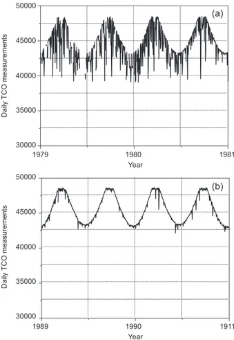
Figure 1 shows the number of measurements re-corded at the beginning of the TOMS campaign from Nimbus-7. It depicts a double interannual periodicity. The maxima denote maximum satellite coverage and correspond to the spring and fall equinoxes (late March and late September, respectively). Minima occur near the summer and winter solstices (late June and late December). A high variation can be observed in the measurements from 1978 through 1981 (Fig. 1a) while variation during the following decade (1989-1991) is less prominent (Fig. 1b). Variation reflects the discrepancy between the number of parcels measured and the total number of parcels, due to the satellite’s inability to maintain a 100% coverage.
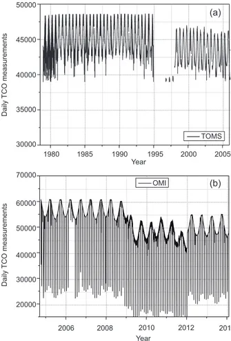
Figure 2 presents the variation in the number of TCO daily measurements number throughout the sat-ellite campaign from 1978 to 2014. Figure 2a shows TOMS measurements, while Figure 2b shows OMI measurements. The TOMS campaign onboard Earth Probe (1996-2007) had much lower coverage than the campaigns onboard Nimbus-7 (1978-1993) and Meteor-3 (1991-1994). Figure 2b shows an excellent OMI coverage between 2004 and mid-2009, although the subsequent variation was higher.
The Earth’s surface was divided in 51800 parcels for TOMS, which operated onboard Nimbus-7 and Meteor-3 from 1978 to 1991. During this time the average number of measured parcels and its standard deviation was of 45 310 ± 2064. After the 1994 failure
of Meteor-3, the next gathered data were erratic num-bers of measurements onboard Earth Probe (1996-1997). From 1998 to 2004 Earth Probe gathered an average of 43 381 ± 1965 measurements (about 1900 measurements lower than Nimbus-7 and Meteor-3).
In the case of OMI, between 2004 and 2009, from a total of 64 800 parcels in which the land surface is divided, the average number of recorded measurements was 56 191 and its standard deviation ±3047. As can be seen in Figure 2b, between 2010 and 2012 the mean number of recorded measurements decreased around 15%.
Two periods of total ozone mass trends analysis were defined for this paper, in accordance with data availability and the stipulation of covering full years. From Figure 2, it is evident that the periods appro-priated to assess total ozone mass are 1979-1991 and 2004-2009. The first period coincides with the
50000
(a)
(b) 45000
40000
35000
30000
1979 1980
Year
1981
1989 1990
Year
1911
Daily
TCO measurement
s
50000
45000
40000
35000
30000
Daily
TCO measurements
greatest and extending damage of the ozone layer. The second period coincides with the so-called ozone layer stabilization phase.
3. Total mass of atmospheric ozone
3.1 Simplified quantification using the typical TCO value (300 DU)
A simple way of quantifying the atmospheric ozone total mass can be derived from the typical TCO val-ue (300 DU) (Rowland et al., 1988). By definition, 1 DU is equivalent to 2.69 × 10¹⁶ molecules of ozone
in a 1 cm2 column. The conversion of the TCO
typ-ical value (300 DU) to the corresponding number of molecules, multiplied by the area of the Earth’s surface, results in the total number of molecules in the atmosphere:
N(O3) = TCO (DU)×2.69
× 1016 O3 molecules
cm2 DU * AT (cm2)
(
)
Using the volumetric mean radius of the Earth (6371.008 km) (NASA, 2010) the total number of O3
molecules corresponding to the average TCO typical value is 4.116 × 1037. The O
3 molecules fraction
corresponding to the typical TCO value can be easily calculated from the total atmosphere mass, which is 5.1352 × 10¹⁸ kg (Trenberth, 2004). The total num-ber of air molecules is 1097 × 1044. Then, to obtain
the molecule fraction of atmospheric O3, the number
of ozone molecules is divided by the total number of air molecules, resulting in 3.75 × 10⁻⁷.
The atmospheric ozone total mass w(O3) is equal
to the total number of ozone molecules N(O3)
multi-plied by the ozone molecular weight and divided by Avogadro’s number NA. The total mass of ozone is
w(O3) =
= 3.32 × 10¹² kg
N(O3)(molecules) * M(O3) (g/mol)
NA (molecules/mol)
However, this value may be far from reality, since it assumes that the typical TCO value is constant over the entire Earth. Actually, TCO varies seasonally and depends strongly on latitude.
3.2 Total ozone mass quantification using TOMS and OMI data
TOMS and OMI files contain an assembly of mea-surements encompassing daily TCO levels over the entire Earth. Therefore, they provide an opportunity to directly quantify the total amount of atmospheric ozone. This requires converting TCO data (DU) to the corresponding ozone amount, either in ozone molecules number or in total mass.
To calculate the number of ozone molecules for each parcel Ni, we simply multiply the TCO value for
each parcel by the conversion factor (1 DU = 2.69 × 10¹⁶ ozone molecules per cm2) and multiply the result
by the surface area of each parcel Ai:
Ni = TCO (DU) * 2.69×10¹⁶
* Ai (cm2)
)
(
O3 moleculescm2 (a)
(b) 50000
45000
40000
35000
30000
Daily
TCO measurement
s
70000
60000
50000
30000 40000
20000
Daily
TCO measurement
s
2006 2008 2010 2012
Year
1980 1985 1990 1995 2000 2005
Year
2014 TOMS
OMI
It is important to keep in mind that parcels vary in surface area (as a function of latitude ϕ at which they are located) and that TOMS parcels measure 1.25º longitude by 1º latitude while OMI parcels measure 1º longitude by 1º latitude.
In the case of TOMS, the surface area of each parcel is
Ai= cos |ø| 2
(2πRT)
288 × 360
While for OMI the surface area of each parcel is
Ai= cos |ø| 2
( )
2πRT360
RT is the radius of the Earth, and ϕ (–90º < ϕ < 90º)
is the latitude of the parcel, being 288 the number of bins by latitude for TOMS and 360 the number of bins by latitude for OMI.
The ozone mass over each parcel can be calculated using the ozone molecular weight and Avogadro’s number NA, this is
mi= Ni(ON3molecules) * M (g/mol) A (molecules/mol)
Then, the total ozone mass is the sum of the mass-es over each parcel:
MT =
∑
mi3.3 Trends of global and hemispherical ozone mass using TOMS and OMI data
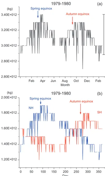
Figure 3a shows the interannual changes of the global mass of ozone in the first full year of TOMS measurements onboard Nimbus 7. It depicts the double interannual periodicity. In Figure 3b the hemispherical contribution to the total mass of ozone is noted. It can be easily inferred that its first maximum is due mainly to the contribution of the Northern Hemisphere, while the second to that of the Southern Hemisphere.
Variable coverage is a problem involved in cal-culating the total ozone amount from TOMS and OMI measurements. It results from two types of data absences, one derived from the low lighting in Polar regions, and the other from faults in measurements. In our study, failed measurements were interpolated and missing data from the Polar regions were omitted.
This approximation includes only the measurable, photo-exposed ozone.
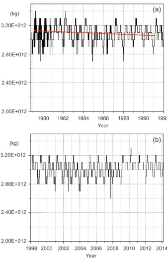
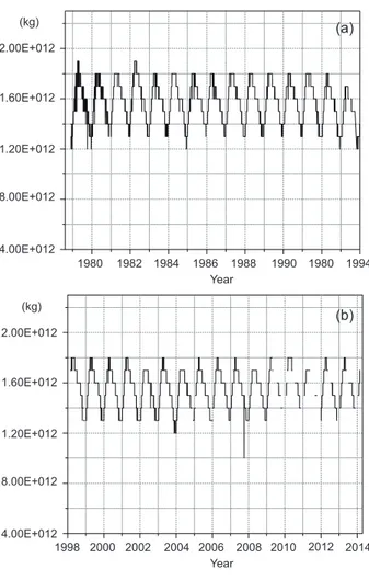
Figure 4a shows the photo-exposed or active glob-al ozone mass derived from TOMS measurements for the period 1978-1994. It highlights a significant decline during 1992 and 1994, which is probably due to data underestimation. As stated above, the mass calculations took into account only days with a number of measurements greater than 75% of the observable parcels; hence, the absence of a number of data undoubtedly influences the total quantification. For this reason, data from 1992, 1993, and 1994 are excluded from the calculations.
Feb Apr
1979-1980 (a)
1979-1980 (b)
Jun
MonthAug Oct Dec Feb (kg)
3.40E+012
3.20E+012
3.00E+012
2.80E+012
2.80E+012
(kg) 2.00E+012
1.80E+012
1.60E+012
1.40E+012
1.20E+012
Spring equinox
Autumn equinox SH
50
0 100 150 200 250 300 350
Day NH
Spring equinox
Autumn equinox
The interannual variations show two peaks per year, whose maxima correspond to the spring and fall equinoxes. The first maximum is due to the contribution of the Northern Hemisphere and the second maximum to the contribution of the Southern Hemisphere. The mass of total ozone in the period 1978-1991 (excluding the years 1992-1994) ranged annually from 2.7 × 10¹² to 3.4 × 10¹² kg, with an
average value of 3.10401 ± 0.11405 × 10¹² kg.
The seasonal change of the total atmospheric ozone mass, or the difference between maximum and minimum values, averaged 20.6% of the maximum values present at the equinoxes. Seasonal variations apply only to measured or photo-exposed ozone. The unmeasured region near the poles can extend to 29º latitude at the solstices, covering 6.269% of the
Earth’s surface. At the equinoxes, the unmonitored area reaches only 6º latitude, covering 0.5478% of the Earth’s surface. The total ozone mass measured during the equinoxes is close to the real value, so there is no need to interpolate the poorly lit Polar regions.
Assuming that the ratio of unmeasured to total ozone corresponds to the ratio of unmonitored to total area, we estimated global ozone at 3.4186 × 10¹² kg in the
equinoxes and 2.86926 × 10¹² kg in the solstices. The
difference of 0.54936 × 10¹² kg represents
approxi-mately 16% of the maximum total ozone.
The linear fit between November 1978 and November 1991 shows a global ozone decrease of 4.72063 × 10⁹ kg per year, representing a loss of
0.1509% per year or 1.509% per decade (3.92% in 26 years).
Figure 4b shows the behavior of the ozone total mass for the period 1998 to 2014. The two peaks per year continue to appear. The second annual peak, which corresponds to the Southern Hemisphere, is quite smaller, which is an evidence of a more severe deterioration resulting from the amplification of the ozone layer hole. Figure 4b also shows very low values in TOM measurements and discontinuities after 2008. The first ones are due to the absence of data or registration of zeros in many daily files; the discontinuities are due to the absence of the complete files. In fact, the frequency of a limited number of data can be seen in Figure 2b. Consequently, OMI years 2009-2014 were excluded from both the ozone mass average value calculation and the linear fit.
The photo-exposed or active global ozone mass in the period 2004-2008 varied annually from 2.6 × 10¹²
to 3.2 × 10¹² kg, with an average value of 2.98923
× 1012 ± 0.091558 × 10¹² kg. In this period, growth
was recorded at an increment of 2.0307 × 10⁹ kg per
year, or 0.016228% per year with respect to 1978 (0.16228% per decade).
Another way to evaluate the global ozone mass decrease is comparing the average annual value at the start of satellite measurements with the average value of one year in stability. Between November 1978 and November 1979, the first year of the study, the average value of the total mass of ozone standard deviation was 3.1283 ± 0.1337 × 10¹² kg. Between
November 2004 and November 2005, the average value of the ozone mass was 2.9979 ± 0.0917 × 10¹² kg. The difference between 1978 and 2004 was
(a)
(b) (kg)
3.20E+012
2.80E+012
2.40E+012
2.00E+012
(kg)
3.20E+012
2.80E+012
2.40E+012
2.00E+012
1980 1982 1984 1986 Year
1998 2000 2002 2004 2006 2008 2010 2012 2014 Year
1988 1990 1992
1.3033 ± 0.332 × 10¹¹ kg, representing a decrease
of 4.17% in the ozone total mass in 26 years (1.6% per decade).
Both methods for evaluating ozone mass change, linear regression analysis as well as comparison of average values per year from 1978-1979 and 2004-2005, revealed a decrease of the same approximate magnitude, i.e., about 4% in 26 years (1.6% per decade).
Figure 5 shows the behavior of ozone total mass in the Northern Hemisphere. In the period 1978-1991, the ozone mass ranged from 1.2 × 10¹² to 1.9 × 10¹² kg,
with an average value of 1.59426 ± 0.1573 × 10¹² kg.
This means that during this period, 51.34% of global ozone resided in the Northern Hemisphere. The linear fit shows an annual decrease of 1.95026
× 109 kg or 0.1228%, equating to a decrease of
1.228% per decade and 3.2% in the 26-yr period of 1978-2004.
In the period 2004-2008, the ozone total mass in the Northern Hemisphere ranged from 1.0 × 10¹² to
1.8 × 10¹² kg with an average value of 1.54668 ±
0.14151 × 10¹² kg. The difference between the
av-erage value for this period vs. 1978-1991 was 4.758 × 10¹⁰ kg, or 2.98% less than the earlier period. The
linear fit from 2004 to 2008 shows an annual growth of 2.41863 × 10⁸ kg or 0.003909%, equating to an
increase of 0.03909% per decade compared to 2004, which implies stabilization.
Figure 6 shows the behavior of the ozone total mass in the Southern Hemisphere. In the period 1978-1992, the ozone mass ranged from 1.1 × 10¹² to 1.8 ×
(kg) (a)
(b) 2.00E+012
1.60E+012
1.20E+012
8.00E+012
4.00E+012
(kg)
2.00E+012
1.60E+012
1.20E+012
8.00E+012
4.00E+012
1980 1982 1984 1986 1988 1990 1980 1994 Year
1998 2000 2002 2004 2006 2008 2010 2012 2014 Year
Fig. 5. Behavior of the total ozone mass (kg) in the North-ern Hemisphere from TOMS and OMI for the periods (a) 1987-1994, and (b) 1998-2014.
Fig. 6. Behavior of the total ozone mass (kg) in the South-ern Hemisphere from TOMS and OMI for the periods (a) 1987-1994, and (b) 1998-2014.
1980 1982 1984 1986 1988 1990 1980 1994 Year
(kg)
2.00E+012
1.60E+012
1.20E+012
8.00E+012
4.00E+012
(kg)
2.00E+012
1.60E+012
1.20E+012
8.00E+012
4.00E+012
1998 2000 2002 2004 2006 2008 2010 2012 2014 Year
(a)
1012 kg, with an average value of 1.51426 ± 0.11409
× 1012 kg. The linear fit shows an annual decrease of
3.02391 × 10⁹ kg or 0.199695% per year, equating
to a decrease of 1.959% per decade and 5.19% in the 26-year period of 1978 and 2004.
In the period 2004-2008, the total ozone mass of the Southern Hemisphere ranged from 1.3 × 10¹² to 1.6 ×
1012 kg, with an average value of 1.43886 ± 0.09667
× 1012 kg. The difference between the average value
for this period versus 1978-1991 was 7.54 × 10¹⁰ kg,
or 4.98% less than the earlier period. During the period 2004-2008 the amplitude of the seasonal variation was almost constant, reinforcing the idea of stabilization. However, recent signs of ozone stabilization fall short of recovery expectations. Severe ozone loss in the Southern Hemisphere, where the second annual peak has almost disappeared from interannual global behav-ior, indicates a dramatic change in ozone distribution between the hemispheres.
4. Conclusions and discussion
Using all daily TCO measurements from TOMS and OMI, we present a method to quantify the ac-tive ozone total amount, i.e., measurable ozone. In the period 1978-1991 the ozone total mass ranged annually from 2.7 × 10¹² to 3.4 × 10¹² kg, with an
average value of 3.10399 ± 0.11406 × 10¹² kg. The
raw amplitude of interannual variations is 20.6% of the maximum value.
The fraction of the unmonitored Earth’s sur-face area is 0.06269 (6.269%) at the solstices and 0.005478 (0.5478%) at the equinoxes. Using the fraction of unmeasured area to correct for unmea-sured ozone, we observe a net interannual variation of the total ozone mass of 16% instead of the 20.6% of gross interannual variation. This net interannual variation is impressive and of course requires an explanation, which for the moment is beyond our scope.
Additionally, the period of 1978-1991 exhibited a decrease in the global total ozone mass of 4.72063 × 10⁹ kg per year, equivalent to a loss of 1.5088%
per decade (1.228% in the Northern Hemisphere and 1.959% in the Southern Hemisphere).
It makes sense to perform a trends analysis in terms of total ozone amount rather than TCO. A previous global and hemispherical study of the
TCO interannual variation has been conducted by our working group (Pinedo-Vega et al., 2017) using all daily TCO measurements from TOMS and OMI, concluding that in the period 1978-1994, global TCO decreased by 4.3% or 13.5 DU per decade (4.05% in the Northern Hemisphere and 4.5% in the Southern Hemisphere). This confirms that the relationship between TCO and ozone mass is not at all linear.
In the period 2004-2008, the global mass of ac-tive ozone varied annually between 2.6 × 10¹² and
3.2 × 10¹² kg, with an average of 2.98923 × 10¹²
± 0.091558 × 10¹² kg. Both linear regression and
comparison of total ozone mass average values per year between 1978 and 2004 yield a global decrease of about 4% in 26 yrs. The Northern Hemisphere, which contains 51.34% of global ozone, experi-enced ozone loss at a rate of 3.2% from 1978 to 2004, while the Southern Hemisphere experienced loss at a rate of 5.09%.
In contrast, between 2004 and 2008 a slight in-crease in the global total ozone mass was recorded: 2.03 × 10⁹ kg or 0.016228% per year compared to
1978. In the Northern Hemisphere, ozone increased by 0.0152% per year, while in the Southern Hemi-sphere it increased by 0.3169% per year. Recent ozone increases have been attributed in part to the solar cycle 23 (Cunnold et al., 2004; Harris et al., 2008).
If the recovery from 2004 to 2008 was caused by solar cycle 23, the issue is that solar cycles are not continuous but periodic. Although this increase is encouraging, the recovery time of atmospheric ozone remains unpredictable. Furthermore, the ozone problem is not confined to a reduction in total mass; there is also the problem of change in the geograph-ical distribution of ozone. Particularly in this work there is evidence that the distribution between hemi-spheres has changed dramatically and is potentially irreversible.
mass reduction. This value of ozone molecules vs. air molecules is lower than the theoretical value (3.75 molecules of ozone for every 10 million molecules of air) calculated from the typical TCO value of 300 DU (section 3.1).
References
Bodeker G.E., Connor B.J., Liley J.B. and Matthews W.A., 2001. The Global mass of ozone: 1978-1998. Geophys. Res. Lett. 28, 2819-2822,
DOI: 10.1029/2000GL012472
Cunnold D.M., Yang E.S., Newchurch M.J., Reinsel G.C., Zawodny J.M. and Russell III J.M., 2004. Comment on ‘‘Enhanced upper stratospheric ozone: Sign of recovery or solar cycle effect?’’ by W. Steinbrecht et al.. J. Geophys. Res. 109, D14305.
DOI: 10.1029/2004JD004826
Dave J.V. and Mateer C.L., 1967. A preliminary study on the possibility of estimating total atmospheric ozone from satellite measurements. J. Atmos. Sci. 24, 414-427. DOI: 10.1175/1520-0469(1967)024<0414:APSOT-P>2.0.CO;2
Harris N.R.P., Kyrö E., Staehelin J., Brunner D., Andersen S.-B., Godin-Beekmann S., Dhomse S., Hadjinicolaou P., Hansen G., Isaksen I., Jrrar A., Karpetchko A., Kivi R., Knudsen B., Krizan P., Lastovicka J., Maeder J., Orsolini Y., Pyle J.A., Rex M., Vanicek K., Weber M., Wohltmann I., Zanis P. and Zerefos C., 2008. Ozone trends at northern mid- and high latitudes – a European perspective. Ann. Geophys. 26, 1207-1220.
DOI: 10.5194/angeo-26-1207-2008
NASA, 2010. Earth fact sheet. Archived from the original on 30 October 2010. Available at: https://nssdc.gsfc. nasa.gov/planetary/factsheet/earthfact.html.
Pinedo-Vega J.L., Molina-Almaraz M., Ríos-Martínez C., Mireles-García F. and Dávila-Rangel J.I., 2017. Global and hemispherical interannual variation of total column ozone from TOMS and OMI Data. Atmos. Clim. Sci. 7, 247-255. DOI: 10.4236/acs.2017.73017