CAVITATION NOISE MODELING AND ANALYZING

CAVITATION NOISE MODELING AND ANALYZING

PACS: 43.25.Yw

Vokurka Karel

Technical University of Liberec Physics Department

Halkova 6

CZ-461 17 Liberec Czech Republic Tel.: 00420-48-5353401 Fax: 00420-48-5353113 E-mail: karel.vokurka@vslib.cz

ABSTRACT. Cavitation noise represents a useful source of information on physical processes accompanying bubble oscillations in liquids. However, to be able to extract this information from measured data, both a suitable mathematical model of cavitation noise and an appropriate method for signal analysis are necessary. In presentation these problems are discussed in detail in view of recent results obtained by the author. Cavitation noise is modeled under assumption that certain parameters controlling the bubble oscillations are random and hence radiated pressure waves, perceived as cavitation noise, may be described as a superposition of nonrandom functions governed by a finite set of random parameters. The mean values of these parameters are obtained from a numerical computation using the Gilmore's model of an oscillating bubble. Cavitation noise model is then used to generate a time series which can be analyzed. The computed autospectral densities are compared with corresponding experimentally determined autospectral densities and inferences on cavitation noise are drawn.

INTRODUCTION

Oscillating cavitation bubbles represent a source of intensive pressure waves. As these waves have a random character, they are called cavitation noise. Cavitation noise is carrying information about the oscillating bubbles and it should be possible, using a proper method of analysis, to extract this information. A number of statistical characteristics can be used for this purpose. However, in experiments, autospectral densities of cavitation noise have been measured first of all [1 - 4].

To be able to extract the information contained in autospectral densities, a suitable physical and mathematical model of cavitation noise is needed. In the literature three approaches to cavitation noise modeling can be found. Cramer and Lauterborn [5] concentrated on explanation of the origin of discrete spectral lines and among them especially on subharmonics and their harmonics. Another approach to this problem has been presented in reference [6], where cavitation noise is explained using a chaos theory. Yet another approach has been considered by Bohn [2], who suggested to use a random pulse processes to model cavitation noise.

CAVITATION NOISE MODELS

When a liquid is irradiated by a sufficiently intensive periodic pressure wave, cavitation bubbles are generated and forced to oscillate. The bubbles grow during strain half-periods of the driving acoustic field and are compressed during stress half-periods. While oscillating, the bubbles emit pressure waves into the surrounding liquid. These pressure waves consist of short, steep, high pressure pulses and of long, moderate, rarefaction portions. The pressure pulses are radiated when the bubbles are compressed to minimum volumes. As this happens during the stress half-periods, the pressure pulses are emitted at almost periodic intervals equal to the period of the driving acoustic field. In the following the rarefaction portion of the pressure wave will be not considered and the pressure pulse form will be approximated by a double-sided exponential function [7]

( )

(

θ

)

1 t P t

p

=

−

Values of the peak pressure P and time constant θ can be estimated using the scaling functions published in reference [8]. These scaling functions have been computed using the Gilmore's model of an oscillating bubble. Assuming the amplitude of bubble oscillations A=3.5 and the adiabatic exponent for the bubble content (vapour) γ=1.25 [7], the corresponding non-dimensional peak acoustic pressure in the pulse is Pz=200, and non-dimensional pulse effective

width ϑz=10

-3

. Assuming further that the maximum bubble radius is RM=1 mm and that pressure

pulse is measured at a distance r=0.1 m from the bubble centre, the dimensional peak acoustic pressure is P=3x105 Pa and pulse effective width ϑ=0.1 µs. These values correspond to water (ρ∞=103 kg.m-3) under atmospheric pressure p∞=105 Pa. It is an easy exercise to verify that for

the pressure pulse form given by equation (1) the effective pulse width ϑ is equal to the time constant θ.

Let us assume that the pressure pulses radiated in different periods are mutually independent (this corresponds to a "bubble without memory"). For reasons which will be clear later two models of cavitation noise will be considered. In the first case a single cavitation bubble is assumed. Then the mathematical model of cavitation noise p(t) can be written in the form [9]

( )

_∑

(

)

−

−

−

=

k

t

kT

P

t

p

exp

ϕ

/

θ

Here Pk is a random peak acoustic pressure of the pulse in the kth period, ϕk is a random

distance of the kth pulse from a reference point in the kth period, and θk is a random time

constant of the pulse in the kth period [9].

In the second case a cavitation field consisting of N bubbles is assumed. Now the pressure pulses are radiated almost synchronously and thus groups of random pressure pulses are arriving almost periodically at the place of a hydrophone. The model of the cavitation noise p(t) can be written now in the form [9]

∑ ∑

−

−

−

=

kT

t

P

t

p

(

)

exp(

/

)

1

θ

ϕ

Here Nk is a random number of pressure pulses in the kth group (period), Pkn is a random

peak acoustic pressure of the nth pulse in the kth group, ϕkn is a random distance of the nth

pulse in the kth group from a reference point in the kth period, and θkn is a random time constant

CAVITATION NOISE ANALYZIS

A closed form formulas for autospectral densities of cavitation noise models defined by equations (2) and (3) have been derived and analyzed in [9]. These closed form formulas are very useful in gaining an insight into the structure of the theoretical autospectral densities, and will be occasionally mentioned in this paper. A different way how to determine the autospectral densities is by simulating cavitation noise (using equations (2) and (3)) on a computer and by computing the corresponding autospectral densities using a standard procedure described, e.g., in [10]. This second approach has been described in reference [11] and will be also used here.

By inspecting the autospectral densities of cavitation noise measured in experiments [1 - 4], it may be seen that they consists of two parts. First, there is an almost flat continuous spectrum, spanning very broad range of frequencies from a few kHz to several MHz [1, 2]. Second, the measured spectra contain discrete lines occurring at a frequency of the driving acoustic field fo,

and its harmonics and subharmonics. The discrete spectral lines exceed the continuous part of the spectrum by about 30 – 40 dB at low frequencies. At higher frequencies the difference between the levels of the continuous and discrete spectra gradually diminishes and at the highest frequencies (approximately >0.7 MHz [1, 2]) only continuous spectrum can be observed. The level of the continuous spectra measured by Tsujino [4] is about 130 dB re 20 µPa.

In order to determine the theoretical autospectral densities, distributions of all random variables in equations (1) and (2) (i.e., N, P, ϕ, and θ) must be specified. First, all the random variables are assumed to be mutually independent. Second, the random variable N is assumed to be Poisson distributed and the random variables P, ϕ, and θ are assumed to be normally distributed. In accordance with the previous section, the mean values of the random variables P and θ are µP=3x10

5

Pa, and µθ=0.1 µs. The frequency of the driving field is fo=20 kHz. As can be

verified, the value of µθ considered here yields a continuous spectrum, which is flat up to approximately 1 MHz. This is in a good agreement with experimentally determined autospectral densities [1, 2].

The remaining mean values and standard deviations have to be selected in such a way as to yield the best match between the theoretical and experimental autospectral densities. An examination of the closed form formulas [9] revealed that the range of frequencies the discrete lines span is basically determined by the standard deviation σϕ of the random variable ϕ. In

order for the spectral lines to sink into the continuous spectrum at a frequency 0.7 MHz, the standard deviation σϕ must be as small as σϕ=0.7 µs. This is a surprising requirement, which is

not easy to interpret in physical terms. For example, to fulfil it, in water, where the speed of sound is approximately c=1450 m.s-1, the diameter of cavitation field d should be of the order d=c.σϕ ≈ 1 mm (otherwise, even if all bubbles in the field are compressed exactly at the same

time, the difference in times the pulses arrive to the hydrophone from the most and least distant bubbles will be larger than σϕ). And this is the reason why the single-bubble cavitation noise

model (2) has been also considered here. But in the case of the single-bubble model, both the continuous and discrete spectra levels lie much lower than determined by Tsujino [4]. To achieve the levels measured by Tsujino [4], a cavitation field consisting of about 50 bubbles has to be considered. Hence, the second model defined by equation (3), with mean value of pulses in groups µN=50, is also used.

The remaining two parameters (σP and σθ) should be assigned values, supporting the

similarities between the autospectral densities. In the case of equation (2), the values σP=5x10

4

Pa and σθ=10 ns have been selected, and in the case of equation (3), they have been σP=10

5

Pa and σθ=50 ns.

Using the distributions and parameters specified above, cavitation noise records consisting of 100 periods have been simulated on a computer with a sampling frequency fs=82 MHz.

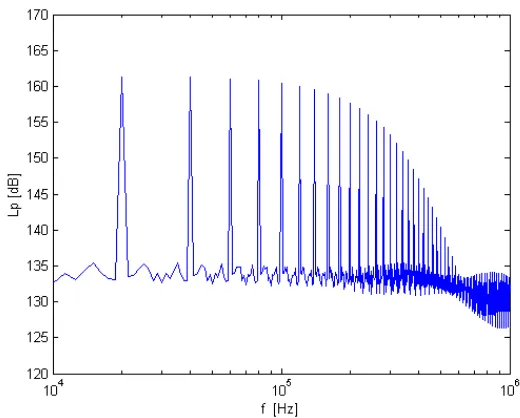
Autospectral densities have been computed for these records with a frequency resolution ∆f=1250 Hz. Number of averages was NA=85. The computed autospectral densities are shown

Fig. 1. Autospectral density of simulated cavitation noise in the case of single-bubble cavitation

Fig. 2. Autospectral density of simulated cavitation noise in the case of multi-bubble cavitation

As can be seen from Figs. 1 and 2, both autospectral densities of simulated cavitation noise match the measured spectra relatively well. The main deviation in Fig. 1 concerns the relatively low levels of both continuous and discrete spectra as compared with values obtained by Tsujino [4]. These low levels are consequence of the assumption of single-bubble model, which evidently is not true in Tsujino's experiments [4].

In Fig. 2 the levels of both the continuous and discrete spectra agree with the levels measured by Tsujino [4] well. Even the mean number of oscillating bubbles (i.e., µN=50) is

CONCLUSIONS

Cavitation noise models based on random pulse processes have been used to simulate cavitation noise records. The values of model parameters have been selected using partly the Gilmore's model (the mean peak acoustic pressure in the pulse, and the mean time constant of the pulse). The values of the remaining parameters have been selected in such a way as to provide the best match between the experimental and theoretical autospectral densities.

The physically unrealistic small standard deviation of the random time distances of pulses from reference points can be overcome by assuming a single-bubble model. However, fields of cavitation bubbles observed in experiments will provide much higher values of the standard deviation. To resolve this discrepancy further research is needed.

The models considered here also do not provide explanation for the subharmonic discrete spectral components and their harmonics. However, it seems that this could be overcome by introducing correlation between pulses occurring in subsequent periods of the driving field. Work on such an improved model is carried out at present time.

ACKNOWLEDGEMENTS

This work has been supported by the Ministry of Education of the Czech Republic as the research project MSM 245100304.

REFERENCES

[1] Esche R: Untersuchung der Schwingungskavitation in Flüssigkeiten. Akustische Beihefte 4, 208-228, 1952.

[2] Bohn L.: Schalldruckverlauf und Spektrum bei der Schwingungskavitation. Acustica 7, 15, 201-216, 1957.

[3] Lauterborn W, Cramer E: On the dynamics of acoustic cavitation noise spectra. Acustica 49, 4, 280-287, 1981.

[4] Tsujino T: Cavitation damage and noise spectra in a polymer solution. Ultrasonics 25, 67-72, 1987.

[5] Cramer E., Lauterborn W.: Zur Dynamik und Schallabstrahlung kugelförmiger Kavitationsblasen in einem Schallfeld. Acustica 49, 226-238, 1981.

[6] Lauterborn W., Parlitz U.: Methods of chaos physics and their application to acoustics. Journal of the Acoustical Society of America 84, 6, 1975-1993, 1988.

[7] Vokurka K.: Experimental study of the bubble pulse. Acustica 66, 3, 174-176, 1988. [8] Vokurka K.: A method for evaluating experimental data in bubble dynamics studies.

Czechoslovak Journal of Physics B36, 5, 600-615, 1986.

[9] Vokurka K.: Power spectrum of the periodic group pulse process. Kybernetika16, 5, 462-471, 1980.

[10] Bendat J., Piersol A.: Random data analysis and measurement procedures. Wiley, New York 1986.