GENERATING REALISTIC VIRTUAL SOUNDS WITH A LIMITED NUMBER OF SPECTRAL FEATURES

GENERATING REALISTIC VIRTUAL SOUNDS WITH A LIMITED NUMBER OF

SPECTRAL FEATURES

PACS REFERENCE: 43.66Ba, 43.66Pn, 43.66Qp

Langendijk, E. H. A.1; Bronkhorst, A. W. TNO-Human Factors

P.O. Box 23, 3769 ZG Soesterberg

The Netherlands Tel: +31-40-2131664 Fax: +31-40-2744675

E-mail: erno.langendijk@philips.com

ABSTRACT

In order to generate realistic virtual sounds optimized to individual listeners it is important to know the spectral localization cues in the directional transfer functions (DTFs). Those cues were identified in two localization experiments, one in which spectral features were distorted and another in which a limited number of features (1-6) were present in the DTFs. The results indicate that realistic virtual sounds can be created with three features in the DTFs. The first primary peak contributes to sound localization above the horizontal plane. The first primary dip and the second primary peak contribute to elevation and front-back discrimination, respectively, below the horizontal plane. Between individuals each feature exists in a limited frequency range.

INTRODUCTION

Usually, when we hear a sound we perceive it as coming from a certain position that coincides with the sound source. The physical sound source and the perceived sound source are one and the same. When we record the sound and play it back over headphones, however, the sound is perceived at a rather strange position, namely inside the head. Yet, by careful manipulation of the headphone signal, such that it mimics the acoustic signal of a free-field sound source at the eardrum, a virtual sound source can be created that is perceived at the same apparent position as the free-field source. The goal of the present study is to investigate what acoustic information is essential to generate realistic virtual sound sources over headphones and herewith to identify what acoustic cues the auditory system uses to localize sounds.

In order to determine the position of a sound source the auditory system has to extract position information from the acoustic signals that arrive at the ears. When a sound is generated to the right of the head it will arrive earlier and have higher amplitude at the right ear than at the left ear. The timing difference - referred to as interaural time difference (ITD) - is mainly caused by the difference in the distance from the sound source to either ear. The amplitude difference – called interaural intensity difference (IID) - is caused by the acoustic head shadow; for the ear that is turned away from the sound source the sound waves are (partly) obstructed by the head, i.e. the acoustic signal is attenuated. These binaural cues vary quite systematically with the lateral (left-right) position of the sound source.

1 _{Present address: Philips Research, Prof. Holstlaan 4, 5656 AA, Eindhoven, The}

For different sound source positions in the median plane (the vertical plane dividing the left and right sides of the head), however, the binaural cues are approximately constant and cannot be used as localization cues. Nevertheless, humans are well able to localize sound sources in the median plane. However, when the pinnae (ear shells) are modified by filling them with putty (e.g. Gardner and Gardner, 1973; Oldfield and Parker, 1984b) or covered with blocks (Gardner and Gardner, 1973) localization accuracy deteriorates drastically. Hence, the pinnae play an important role in localization of sounds in the median plane.

Measurements of the transfer functions from a sound source to the eardrum - called the head-related transfer functions (or HRTFs) - revealed that the pinnae filter the sound in a very characteristic way, introducing large peaks and dips in the spectrum that are unique with respect to the position of the sound source (Blauert, 1969/1970; Shaw, 1982). The variations of these spectra as a function of elevation are, however, rather complex. Apart from that, there are also substantial individual differences (Wenzel et al.,1993), which complicate the investigation of which cues are important for sound localization. Therefore, it is not surprising that despite many research efforts localization of sound sources in the median plane is still not well understood.

The focus of the present study is to investigate what spectral cues human listeners use when localizing sounds.

METHODS

In the present study, a powerful method is used to investigate the contribution of spectral cues to human sound localization. In this method sounds are not presented to listeners via actual loudspeakers placed at certain positions in the free field, but via virtual sound sources generated over headphones.

In order to simulate realistic free-field sound sources over headphones, it is important that the sound field at the eardrum is reproduced correctly. The procedure is described extensively in (Langendijk and Bronkhorst, 2000). In short, generating virtual sounds was accomplished by measuring the transfer function from loudspeaker to eardrum, called head-related transfer function (HRTF), with very small probe-tube microphones that were positioned such that the tips of the probes were within 1-2 mm from the eardrum. Using the same microphones, the transfer function from headphone to eardrum (HPTF) was measured as well. Then, when a sound is filtered for each ear with the HRTF and inverse filtered with the HPTF and presented over the headphones, the acoustic stimulus at the eardrum is (nearly) identical to that of the free field. Consequently, a virtual sound source is perceived at (nearly) the same apparent position as that of the actual free-field loudspeaker.

In order to facilitate the extraction of spectral features from the HRTFs that are important for sound localization, the log-amplitude spectrum of each HRTF was treated as the sum of two functions; the average transfer function (ATF) and the directional transfer function (DTF). The ATF contained non-directional components of the HRTFs such as the ear canal resonance and was calculated by averaging the HRTFs across all measured positions (n=976) for each ear for each listener. The DTFs were calculated by subtracting the ATF from the HRTFs and contained therefore the

direction-dependent components of the HRTFs.

Target stimuli were bursts of 200-ms Gaussian noise bandpass filtered between 200 Hz and 16 kHz with 10-ms cosine square on- and offset ramps. Twenty-five files with noise bursts were stored on a hard-disc of a PC; on each presentation a file was chosen at random, played via a DA converter (Tucker Davis Technologies, DD1) and fed into the DSP-board for real-time filtering. The stimuli were presented via Sennheiser headphones at an A-weighted level of approximately 65 dB.

As a response method a so-called "Virtual Acoustic Pointer" (VAP) was used, such as described by Langendijk and Bronkhorst (2002). In short, the VAP is a virtual sound source whose position can be controlled with a stick that pivots about a fixed point. The VAP plays a pulsed broadband harmonic complex tone, which is a stimulus that can be localized very accurately and which was different from the target stimuli in the experiments (broadband Gaussian white noise). Listeners gave a response by placing the VAP at the same apparent position as the target stimulus. The method is a very accurate one to measure the effect of disturbing localization cues Langendijk and Bronkhorst (1997).

Design

Eight listeners with normal hearing (hearing loss <20 dB, at octave frequencies between 250 and 8000 Hz) participated in each experiment. All listeners had previous experience in sound localization experiments. The authors, who were also subjects, had extensive experience in sound localization experiments.

In the first experiment, spectral cues in specific frequency bands were removed by replacing the corresponding part of the DTF by its average value for that band. The modification was performed separately for the left and right ears. There were nine experimental conditions. In the baseline condition, no spectral cues were removed from the DTFs. In the 2-octave condition, spectral cues were removed from the 4-16 kHz frequency band. In the three 1-octave conditions, referred to as the low, middle and high 1-octave conditions, spectral cues were removed from 4-8, 5.7-11.3 and 8-16 kHz, respectively. In the low, middle-low, middle-high and high 1/2-octave conditions spectral cues were removed from 4-5.7, 5.7-8, 8-11.3 and 11.3-16 kHz, respectively. Figure 1 illustrates how the left-ear DTF of one of the listeners for the direction (azimuth,elevation) is (0,-56) degrees changes when spectral cues are removed from the eight frequency bands. In the experiment, there were a total of 23 target positions evenly distributed in the right hemisphere. The targets were

presented 5 times in each condition in a balanced order.

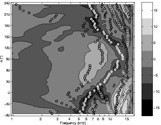
In the second experiment, spectral features that could provide localization cues were identified in the DTFs and the perceptual relevance of each feature for positions in the median plane was investigated in localization experiment. In a semi-automatic procedure the six most prominent spectral features (three peaks and three dips) were marked in the individual DTFs from six listeners. The spectral features were classified using six different categories; #1 first primary peak ())), #2 first primary dip (∃∃), #3 second primary peak (((), #4 second primary dip (∋∋), #5 first secondary peak (++), #6 first secondary dip (,,), respectively. Figure 2 illustrates the features that were labeled in the DTFs of one subject. In the localization experiment, there were thirteen experimental conditions that differed in the processing of the DTF component of the

individually measured HRTFs. In the baseline condition, the raw DTFs were used (i.e. no processing). In the six-feature condition, the DTFs contained the six main features as identified in the feature labeling procedure. From the amplitudes and center frequencies of the features a DTF was constructed by fitting, in the amplitude domain, a half squared-cosine through the amplitudes of each pair of successive features. In the other conditions, one or more features were not present. This was accomplished by replacing the amplitudes of the bins near the feature with the average DTF. That is, if the feature is a peak (dip) then the amplitudes of all bins with an amplitude above (below) the average DTF and with a frequency between the preceding and successive features are replaced with the average DTF.

Because there are as many as 63 unique combinations of creating DTFs with 1 to 6 features a deliberate choice of the features present in each condition was made in order to restrict the number of conditions to 12. The choice was based on the prominence and potential relevance of the features, as determined in the spectral feature analysis. Thus, features with a large absolute amplitude were selected as well as features that could provide unique front-back and/or elevation cues. Most important were considered features #2 and #3, directly followed by #1 and #4, then came feature #5 and finally the least important was considered to be feature #6. In what follows, the name of the condition reflects the features that were present. For example, in the six-feature condition #123456, features #1 through #6 were present in the DTFs. The other conditions were #2, #3 (one-feature conditions), #23, #12, #13, #24 (two-feature conditions), #123, #234, #135 (three-feature conditions), #1234, #2345 (four (three-feature conditions). There were thirteen different target positions in the median plane (both front and rear, with elevations between –60 and +90 degrees). They were presented 6 times in each condition in a random order.

RESULTS

Experiment 1

In order to separate the effects of condition and target position, a repeated-measures analysis of variance (ANOVA) was performed of the elevation error and the percentage of front-back errors. Elevation errors were calculated by taking the absolute difference between target and response elevation, with elevation being the angle with respect to the horizontal plane (i.e. irrespective of front-back location). In the case of front-back errors, the variable of interest was the number of responses in a hemisphere (front or rear) different from that of the target divided by the total number of target presentations. Targets in the lateral-vertical plane were excluded from the front-back analysis. Both types of errors were averaged across the 5 repetitions of each pair of condition and target position. The outcome of the ANOVA showed that all main effects and interactions were significant (p<0.01) for both types of error.

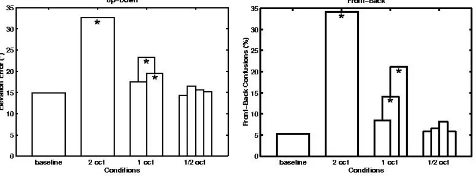
Figure 3: Elevation error (left panel) and percentage of front-back confusions (right panel) in the baseline condition and the other conditions collapsed across listeners and target positions. The width of a bar and the relative position between bars in one condition represents the bandwidth and the relative center frequency of the band in each of the conditions. The * marks conditions significantly different (p<0.05) from the baseline condition.

1-octave conditions were significantly different (p<0.01) from the baseline condition. All three conditions were also significantly different (p<0.05) from each other. The results obtained in the 1/2-octave conditions were not significantly different from those obtained in the baseline condition (p>0.1). The mean elevation error was greatest in the 2-octave condition; it is only somewhat smaller than the mean error of 40 degrees that would have been obtained if listeners had always responded in the direction (0,0) degrees. The fact that the elevation error is significantly greater in the middle 1-octave condition than in the other 1-octave conditions suggests that the up-down cues were most prominent in this frequency region.

The percentage of front-back confusions collapsed across target positions and listeners is shown in the right panel of figure 3. The 2-octave condition and the middle and high 1-octave conditions were significantly different (p<0.01) from the baseline condition, as was tested with a Tukey HSD post-hoc analysis, and each of them was also significantly different (p<0.05) from the other. Differences between the 1/2-octave conditions and the baseline condition were not significant (p>0.1). As with the elevation errors, the mean error was significantly greater in one of the 1-octave conditions - in this case the high 1-octave band - than in the others. This indicates that the front-back cues were located mainly in this band.

Experiment 2

From the raw localization data two types of localization errors were calculated - a front-back error and an elevation error - and an analysis of variance (ANOVA) was performed on each error type. In the case of front-back errors (also referred to as the “percentage of front-back confusions”), the variable of interest was the number of responses in a hemisphere (front or rear) different from the target divided by the total number of target presentations multiplied by one hundred. Front-back confusions, for target-response combinations with either the target or the response within 15 degrees form the lateral-vertical plane (front-back plane), were considered to be due to the natural error variation and therefore not counted as front-back confusions. In the case of elevation errors, the variable of interest was the absolute difference between the target elevation and the response elevation (note that elevation is not affected by front-back confusions).

For each type of error, the results were averaged across target positions in the same region (down-front, up-front, up-back, and down-back where the up/down and front/back regions are separated by the horizontal and lateral-vertical planes, respectively). The data for target positions at 90 degrees elevation were omitted from the analysis.

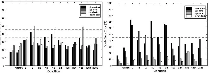
The outcome of the analysis revealed that the effect of condition and the interaction between condition and region, and between subject and region, were significant (p<0.01) for both types of error. For the front-back error also the effect of region was significant (p<0.01). All other effects and interactions were not significant (p>0.2).

The average elevation error and the average percentage of front-back confusions across listeners and positions within regions are plotted in the left and right panels of figure 4, respectively. The results in the right panel indicate that listeners make far more front-back errors for frontal positions than for rear positions. Only for condition #135 a substantial number of front-back errors occur for the rear positions. The data seem

to suggest that if feature #3 is missing in a condition (#2, #12, #24) errors in the down-front region are larger than when this feature is present. In contrast, missing feature #1 seems to affect mostly front-back accuracy in the up-front region (compare conditions #2, #3, #23, #24, #234 and #2345 with the other conditions).

The elevation error is smaller in the two up regions than in the two down regions and it is the highest when the first primary dip (feature #2) is missing in a condition (e.g. #3, #13, and #135). Although this feature seems to be a very important cue for elevation discrimination it is not sufficient for correct localization when present alone (see results condition #2). Localization performance comparable to that in the baseline condition only occurs for conditions with three or more features for which, apart from the first primary dip, also the first and second primary peaks (features #1 and #3, respectively) must be present.

While the first primary dip (feature #2) is the most important elevation cue for positions below the horizon, also the second primary peak (feature #3) seems to have a contribution for those positions, but only when presented together with the first primary dip. For positions with elevations above the horizontal plane the first primary peak (feature #1) seems to be the most important (compare, for example, the results for conditions #123 and #1234 with those for conditions #234 and #2345).

DISCUSSION

The results of the first experiment show that the spectral cues in the 4-16 kHz frequency bands are essential for correctly localizing broadband sounds. The results of the 1-octave conditions suggest that the most important up-down cues are present in the middle 1-octave band (5.7-11.3 kHz) and that front-back cues are coded mainly in the high 1-octave band (8-16 kHz). The results of the second experiment show that for positions in the median plane realistic virtual sounds can be generated using DTFs that contain only

three spectral features: the first primary peak (#1), the first primary dip (#2), and the second primary peak (#3). The first primary peak seems to code both elevation and front-back discrimination for positions above the horizontal plane. For positions below the horizontal plane the first primary dip seems to code elevation discrimination and the second primary peak seems to code front-back discrimination. Other features, such as low-frequency spectral information (below the center frequency of the first primary peak) and secondary peaks and dips at high frequencies (above the center frequency of the first primary dip) can be omitted without affecting localization performance significantly. This suggests that the center frequencies and the amplitudes of the major features provide sufficient information to reconstruct the DTFs for the generation of realistic virtual sounds.

REFERENCES

Blauert, J. (1969/70). “Sound localization in the median plane,” Acustica, 22, 205-213.

Gardner, M.B., and Gardner, R.S. (1973). “Problem of localizing in the median plane: Effect of pinnae cavity occlusion,” J. Acoust. Soc. Am., 53, 400-408.

Langendijk, E.H.A., and Bronkhorst, A.W. (1997). “Collecting localization responses with a virtual acoustic pointer,” J. Acoust. Soc. Am, 101, 3106.

Langendijk, E.H.A., and Bronkhorst, A.W. (2000). “Fidelity of three-dimensional-sound reproduction using a virtual auditory display,” J. Acoust. Soc. Am, 107, 528-537.

Langendijk, E.H.A., and Bronkhorst, A.W. (2002). “Contribution of spectral cues to human sound localization,” J. Acoust. Soc. Am, (Accepted).

Oldfield, S.R., and Parker, S.P.A. (1984). “Acuity of sound localization: a topography of auditory space. II. Pinna cues absent,” Perception, 13, 601-617.

Shaw, E.A.G. (1982). Localization of sound: Theory and Applications, chap. External ear response and sound localization, pp. 30-41. Amphora Press, Groton, CT.