Essays on the Macroeconomics of Labor
Markets
Paula Garda
TESI DOCTORAL UPF / ANY 2013
DIRECTOR DE LA TESI
Prof. Thijs Van Rens. Departament of Economics, University of
Warwick
TUTOR DE LA TESI
Acknowledgments
This dissertation would not have been possible without the help and support
from many. Foremost, I would like to express my deepest gratitude to my
advi-sor Thijs Van Rens for his guidance, advice, and encouragement throughout the
entire project. Special thanks also to Albrecht Glitz for his help, and discussions
that very much helped to improve this thesis.
For further comments on different stages of this thesis I thank Regis
Barni-chon, Vasco Carvahlo, Jordi Gali, Libertad Gonzalez, Kristoffer Nimark,
Bar-bara Rossi, and all the participants of the CREI Macroeconomics Breakfast, and
the UPF Labor, Public and Development Lunch Seminar. I would like to thank
my co-author, Regis Barnichon, for his collaboration on a chapter of this thesis.
Isabel, Lien, and Tomaz supported me with countless discussions along the way.
All of them deserve my gratitude for the help in shaping my thinking about the
topics presented here.
I am grateful to Marta Araque for her patience and invaluable help with
“ev-erything you need”. I am also indebted to the Generalitat de Catalunya for their
financial support.
I also thank my colleagues from cinve for the great support in many different
ways from the very beginning of my post-graduate studies and during all these
years. Because they are “guilty” of my decision to start postgraduate studies.
All this years of research would not have been enjoyable without my friends
in Barcelona. Their company was fundamental. Special thanks to my friends in
Uruguay, who despite the distance, provided my with invaluable support during
all these years.
Finally, I wish to thank my family and extended family. Specially, my mum,
sisters, and my grandparents for their love, encouragement and unconditional
support. Last but certainly not the least, I would like to thank Giorgio, who
experienced all the goods and bads in my life and research during the last four
years, for his unconditional love and support he gives me all the time and because
we are starting a new stage in our live that will probably be more challenging.
Without all of them this journey would have been impossible.
Abstract
This thesis sheds light on several macroeconomic aspects of labor markets. The first chapter focuses on the impact of dual labor markets on human capital investment. Using a large dataset of the Spanish Social Security the wage losses of permanent and fixed term workers after displacement are analyzed. Results indicate that workers under per-manent contracts accumulate a higher share of firm specific human capital than workers under fixed term contracts. The impact on aggregate productivity is analyzed using a calibrated model à la Mortensen and Pissarides (1994) with endogenous investment in human capital and dual labor markets. The second chapter develops a model in order to explain cross countries differences in the cyclical fluctuations of informal employment for developing countries. The explanation can be found in institutional differences be-tween the formal and informal sector. The third chapter proposes a model that uses the flows into and out of unemployment to forecast the unemployment rate. It shows why this model should outperform standard time series models, and quantifies empirically this contribution for several OECD countries.
Resumen
Foreword
This dissertation consists in three self-contained chapters that deal with different aspects of the macroeconomic analysis of the labor markets. The first chapter is concerned about the impact of dual labor market institutions on the investment of human capital and on productivity. The second chapter deals with the cyclical fluctuations of informal em-ployment in developing countries. Finally, the last chapter analyzes the performance of a novel model that uses the flows into and out of unemployment to forecast the unem-ployment rate in OECD countries.
The objective of the first chapter is to evaluate the impact of dual labor market in-stitutions on the investment in firm specific human capital and productivity. Empirically this is done by estimating the impact of mass-layoffs on subsequent wages in Spain, differentiating between workers holding permanent and fixed term contracts at the time of displacement. The main empirical finding is that permanent contract (PC) workers suffer larger and more persistent wage losses than their fixed term contract (FTC) coun-terparts. Wage losses for PC workers stem mainly from the loss of pre-displacement firm tenure, while this source is not important for FTC workers. This is taken as evidence of the difference in the accumulation of job specific human capital between the two type of contracts. The wage loss gap due to the difference of investment in firm specific human capital is estimated to be 6% after the first quarter of displacement. A search and match-ing model à la Mortensen and Pissarides allowmatch-ing for endogenous accumulation of firm specific human capital and the existence of the two type of contracts is developed. The model shows that firms always offer fixed term contracts if they are allowed to do so. The employee’s decision of investment in human capital depends on the expected dura-tion of the contracts, and hence on the expiradura-tion rate of FTC and firing costs. Calibrated to the Spanish economy the model predicts that only PC workers invest in firm specific human capital, while FTC workes do not. This implies that PC workers are on average 12% more productive than FTC. The model suggests that aggregate labor productivity would increase due to the investment in firm specific human capital of FTC workers if the employment protection law for FTC workers was more stringent (i.e. lower maxi-mum duration of this type of contract).
employment in developing countries. Developing countries, as developed ones, are char-acterized by procyclical employment rates, countercyclical unemployment rates. While informal employment asa share of total employment is countercyclical, the cyclical behavior of informal employment in absolute terms (as a percentage of working age population) differs across countries. While in Mexico informal employment inabsolute
termsis countercyclical, in Brazil it has a procyclical behavior. This chapter analyzes
whether institutional differences between the formal and informal sector are important to explain the different cyclical fluctuations of informal employment across countries. In the model, the informal sector arises because of the possibility of evading the pay-ment of a fixed cost that formal firms pay to the governpay-ment. On the other hand, being informal requires bearing the risk of being monitored by the government with the con-sequence of destroying the match, and suffer from lower productivity. Results show that this very simple model can replicate the correlation of informal employment and unem-ployment with output in the case of Mexico and Brazil. The calibration exercise predicts that informal employment as ashareof total employment is countercyclical as in the data. While informal employmentin absolute termsis countercyclical in Mexico, it is procyclical in Brazil. This different cyclical fluctuations of informal employment are driven by a higher productivity gap and higher fixed cost of the formal sector compared to the informal sector, in Mexico relative to Brazil.
Contents
Abstract . . . 5
Foreword 7 Index of tables 5 Index of figures 7 1 WAGE LOSSES AFTER DISPLACEMENT IN DUAL LABOR MARKETS. THE ROLE OF FIRM SPECIFIC HUMAN CAPITAL. 9 1.1 Introduction . . . 9
1.2 Related literature . . . 12
1.3 Data and empirical methodology . . . 15
1.3.1 Data: Continuous Sample of Job Histories . . . 15
1.3.2 A glance at the data . . . 16
1.3.3 Methodology . . . 18
1.4 Empirical results . . . 19
1.4.1 Wage losses after displacement . . . 19
1.4.2 Decomposition of wage losses . . . 20
1.5 A model of dual labor markets and firm specific human capital . . . 23
1.5.1 Match surplus and wage bargaining . . . 25
1.5.2 Job creation and job destruction . . . 25
1.5.3 The workers’ decision of investment in firm specific human capital 27 1.5.4 Wage losses in the model . . . 29
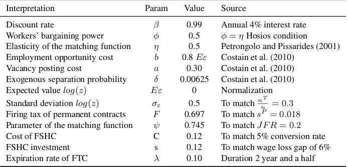
1.6 Calibration and results . . . 30
1.6.1 Calibration . . . 30
1.6.2 The investment decision . . . 31
1.6.3 Wage loss gap in the calibrated model and the data . . . 33
1.6.4 The labor productivity loss . . . 34
1.7 Concluding remarks . . . 34
1.8.1 Sample selection . . . 48
1.8.2 Definition of displacement . . . 49
1.9 Appendix B: Robustness checks . . . 50
1.9.1 Estimation with specific time trends . . . 50
1.9.2 Wage losses by transitions . . . 50
1.10 Appendix C: Surplus functions of the model . . . 54
1.10.1 Fixed Term Contracts surplus . . . 54
1.10.2 Permanent Contract Surplus . . . 54
1.10.3 Steady state equilibrium conditions . . . 55
1.10.4 Steady state employment . . . 55
2 INFORMAL EMPLOYMENT OVER THE BUSINESS CYCLE 59 2.1 Introduction . . . 59
2.2 Informal employment: huge dimensions and cyclical fluctuations . . . . 62
2.2.1 Definition and measure of informal employment . . . 62
2.2.2 Informal employment and cyclical fluctuations . . . 63
2.3 Related literature . . . 65
2.4 A two sector model . . . 66
2.4.1 The main idea . . . 66
2.4.2 Setup of the model . . . 68
2.4.3 Equilibrium . . . 70
2.4.4 Determinants of the size of the informal and formal sector and unemployment . . . 72
2.5 Analyzing the properties over the business cycle: Steady state elasticities 73 2.5.1 A zero productivity gap . . . 74
2.5.2 A positive productivity gap . . . 77
2.5.3 Other parameters . . . 78
2.6 Calibration and simulation results . . . 81
2.6.1 Parametrization of the baseline model . . . 81
2.6.2 Simulation results . . . 82
2.7 Robustness checks . . . 84
2.7.1 Sector specific productivity shocks . . . 84
2.7.2 Wage rigidities in the formal sector . . . 85
2.7.3 Job-to-job transitions between sectors . . . 85
2.7.4 Directed search . . . 86
2.8 Concluding remarks . . . 87
3 THE INS AND OUTS OF FORECASTING UNEMPLOYMENT ACROSS
COUNTRIES 97
3.1 Introduction . . . 97
3.2 Using labor force flows to forecast unemployment . . . 99
3.2.1 The law of motion for unemployment . . . 100
3.2.2 Forecasting labor force flows . . . 101
3.3 Theoretical forecasting performance . . . 102
3.3.1 The AR(1) representation of unemployment dynamics . . . 102
3.3.2 Performance relative to standard time series models . . . 104
3.3.3 Innovation forecasting . . . 104
3.3.4 Misspecification . . . 108
3.3.5 Measurement error and noise-to-signal ratio . . . 109
3.4 Data . . . 110
3.5 Empirical forecasting performance . . . 111
3.5.1 SSUR specification . . . 111
3.5.2 Alternative forecasts . . . 112
3.5.3 Forecast Errors . . . 112
3.5.4 Forecasting Performance over the Business Cycle . . . 114
3.6 Concluding remarks . . . 114 3.7 Appendix: Hazard rate time series properties and Model specifications . 124
List of Tables
1.1 Sample characteristics . . . 36
1.2 Sample characteristics of displaced and non-displaced workers . . . 37
1.3 Differences among displaced workers depending on the type of contract 38 1.4 Determinants of wage losses . . . 39
1.5 Contribution of each determinant to the earning losses . . . 40
1.6 Calibration . . . 40
2.1 Share of informal employment . . . 89
2.2 Cyclical fluctuations in Mexico and Brazil . . . 90
2.3 Parameter configuration . . . 90
2.4 The case of no productivity gap . . . 91
2.5 Simulation results for Mexico and Brazil . . . 92
2.6 Alternative calibration for Mexico and Brazil . . . 93
2.7 Simulation for Brazil: specific productivity shock . . . 94
3.1 Data availability . . . 116
3.2 Unemployment Rate Forecasts. RMSE of SSUR (percentage points) and Relative RMSE to SSUR . . . 117
3.3 Annual unemployment rate forecasts of SSUR and OECD. RMSE (pp) of SSUR and Relative RMSE . . . 118
3.4 Time series properties . . . 124
3.5 ARIMA models for the UR . . . 124
List of Figures
1.1 Wage path of displaced workers in 2001 . . . 41
1.2 Wage losses from separation by type of contract . . . 42
1.3 Wage losses from displacement for low tenured workers . . . 43
1.4 Wage loss gap after controlling for changing industry and unemploy-ment duration . . . 44
1.5 Investment decision in the model . . . 45
1.6 Wage loss gap in the calibrated model and data . . . 46
1.7 Average productivity in the model . . . 47
1.8 The wage loss gapδkwith time specific trends . . . . 51
1.9 Wage losses among different transitions . . . 52
1.10 Wage losses from displacement: different transitions among permanent workers. . . 53
3.1 Average in - and outflow rates across countries . . . 119
3.2 Unemployment rate and conditional steady state unemployment rate . . 120
3.3 Convergence rates to the SSUR . . . 121
3.4 In and Outflows from unemployment . . . 122
Chapter 1
WAGE LOSSES AFTER
DISPLACEMENT IN DUAL
LABOR MARKETS. THE
ROLE OF FIRM SPECIFIC
HUMAN CAPITAL.
1.1
Introduction
In the period 1996-2007, the Spanish economy experienced significantly weaker labor productivity growth than other OECD economies and failed to catch up with the most advanced economies. According to Mora Sanguinetti and Fuentes (2012), the key factor explaining this poor performance is the reduction of TFP growth during this period. This weakening productivity performance in Spain is not explained by specialization in indus-tries with generally weaker productivity growth is several OECD counindus-tries; productivity growth in Spain was relatively weak in a wide range of sectors. The authors identify some characteristics of the Spanish institutional environment that have contributed to the low TFP growth.
con-tracts (FTC) with very low or no employment protection1. These large differences in employment protection lead to a widespread use of fixed-term contracts, reducing train-ing motivations for workers and firms, and discouragtrain-ing investments in firm-specific human capital having detrimental effects on productivity (Damiani and Pompei (2010)). The main objective of this chapter is to investigate the impact of dual labor market institutions on the accumulation of firm specific human capital (FSHC). Therefore, this chapter analyses wage losses after displacement distinguishing between workers holding fixed term and permanent contracts. After displacement, workers usually need to restart their career from scratch in a new job, where they need to acquire new skills or estab-lish a new network inside the firm, with the subsequent wage losses. The acquisition of specific skills through, for example, learning-by-doing on the job and investments in specific training can yield substantial wage losses when starting a new job after dis-placement. Topel (1990) and Neal (1995), and more recently Davis and Wachter (2011), among others, argue that specific forms of human capital play a central role in determin-ing the magnitude of earndetermin-ings losses associated with job displacement.
The first contribution of the chapter is to develop a detailed picture of the displace-ment event in Spain, providing evidence on wage losses after displacedisplace-ment distinguish-ing between displacement from fixed term contracts and permanent contracts. Spain is, in fact, a good laboratory to analyze the sources of wage losses since it is an an ex-treme example of dual labor markets allowing us to analyze the sources of wage losses by type of contract. PC and FTC workers have very different expected job duration. The standard human capital theory of Becker (1964) has clear predictions on the type of human capital accumulated by workers hired under these two different contractual arrangements. PC workers are expected to accumulate more firm specific human capital relative to workers employed with FTC, due to the lower expected duration of the jobs of the latter. Hence, FTC workers wage losses upon displacement should be relatively lower than PC workers’ losses, generating awage loss gapbetween PC and FTC work-ers.
This study makes use of a novel data set that traces the labor market experiences of a large number of workers, and data from their employers in Spain from 1996 to 2008. The resulting data set contains quarterly earnings histories for a large number of dis-placed and non-disdis-placed workers, and the type of contract they hold. Therefore, this chapter reveals a detailed decomposition of the wage losses into firm or sector specific human capital, and unemployment duration.
1
The methodology focuses on mass-layoffs in order to isolate the group of workers who would not have moved under normal business conditions, approximating an ex-ogenous displacement. By doing so, the selection bias problem due to low qualified workers being laid off is reduced. The methodology used is a differences-in-differences approach. Assuming that selection into mass-layoffs is done based on observable pre-displacement characteristics and fixed effects, results show the causal effect of a mass-layoff on wages. The control group is defined by workers not suffering mass-mass-layoffs in the entire period.
The results show that workers under PCs suffer larger and more persistent wage losses after displacement than their fixed term counterparts. In the first quarter after dis-placement PC workers suffer a sharp drop in wages amounting to 20% relative to the control group, consisting of employees not suffereing mass-layoffs in the entire period. While the estimated wage loss for FTC workers, one quarter after displacement, is 8%. In the fourth year following displacement, substantial recovery occurs and the wage loss is estimated 11% average for PC workers and 1% for FTC workers. Results are robust for workers with less than three years of firm tenure. Even if the point estimates are lower for PC workers, there is still a statistcally significant wage loss gap.
In a second step, a decomposition of these wage losses into its sources is done. Re-sults indicate that changing industry has a negative impact on post-displacement wages for both worker types, being the impact of similar size. On the other side, unemployment duration is important to explain wage losses, and is more important for PC workers. Fi-nally, while pre-displacement tenure is the most important source explaining wage losses for PC, it is not important for FTC workers. This is taken as evidence of lower accumu-lation of FSHC under fixed term contracts. The wage loss gap due to the difference in investment in FSHC is 6% in the first quarter after displacement.
In the model, it can be shown that firms always offer FTCs when first matched to workers if legally allowed to do so. Hence workers always begin a match with a FTC. Some of them are going to be converted to a PC, while others will be laid-off. The decision of acquiring human capital will depend on two parameters that determine the duality of the economy: firing costs of PC and the expiration rate of fixed term contracts. Under fixed term contracts there is little incentive to invest in firm specific human capi-tal, since the expected duration of these jobs is not enough to reap the benefits from the investment.
Calibrated to the Spanish economy, the model predicts that only PC workers invest in FSHC, while workers holding FTC do not. In fact, FTC workers invest only if the maximum duration allowed for these contracts is shorter, i.e. stringent law employment protection of FTC workers. This is because with shorter duration of FTCs firms rely less on FTC, converting them more to PC, because laying-off a worker and hiring an-other one is also costly. The 6% wage loss gap due to the difference in the investment in firm specific human capital found in the data, translates into a 12% gap in productivity between the two types of workers. Lastly, the model is used to measure the labor produc-tivity loss due to the use of fixed term contracts with lower investment in firm specific human capital. The model predicts an increase of 16% in aggregate labor productivity if the law on FTC was more stringent, i.e if the maximum duration of FTC goes from two years and a half to two years.
The chapter is organized as follows. The next section revises the related litera-ture. Section 3 presents the empirical analysis, showing the data, and methodology used, while section 4 presents the empirical results. Section 5 presents the theoretical model, and section 6 discusses the results from the model. At the end, conclusions are drawn.
1.2
Related literature
This study is related to three different strands of literature. First, the literature that revises the effects of firing costs, or more general employment protection, on the economy. Sec-ond, the empirical literature documenting earning losses after displacement. And third, search and matching models introducing flexibility at the margin.
analyze employment protection when applied uniformly to all workers in the economy. Studies analyzing the effects of the introduction of flexibility at the margin, i.e. duality, have found that it has created inefficient labor turnover (Boeri (2011))) although the ef-fect on unemployment is mixed, it has increased the volatility of unemployment (Costain et al. (2010), Sala et al. (2011),Bentolila et al. (2010)).
Finally, this research is very related to studies that analyze the effects of dual labor markets on productivity. Damiani and Pompei (2010) look at how employment contacts (permanent and temporary) affect cross-national and sectoral differences in multifac-tor productivity growth in sixteen European countries from 1995 to 2005. The authors show that fixed-term contracts, may discourage investment in skills and have detrimen-tal effects on multifactor productivity increases, and that employment protection reforms which slacken the rules of fixed-term contracts cause potential drawbacks in terms of low productivity gains. Dolado et al. (2012) show that duality institutions have a negative effect on TFP development at the firm level. With a simple model they show that a larger firing cost gap has negative effects on firms’ TFP, by lowering the exerted effort of temporary workers and the training they receive from employers. The authors test this implication by using a longitudinal firm-level dataset. They evaluate the impact of changes in the firing-cost gap on firms’ TFP using as natural experiments several labor market reforms entailing changes in EPL in 1994, 1997 and 2002. They found that firms with larger share of FTC workers before the reforms, show higher conversion rates and higher TFP after the reforms. This chapter looks to the same issue from a different an-gle. First, shows empirically the different content of firm specific human capital between the two type of contract arrangements. Then, shows how this translates to lower labor productivity using a search and matching model with endogenous firm specific human capital investment.
The empirical evidence for Europe is relatively sparse. Studies by Lefranc (2003) for France, Carneiro and Portugal (2006) for Portugal, Eliason and Storrie (2006) for Sweden find the long-term losses to be large and concordant with the earlier studies for the US. Other results for Germany, confirm these findings. Burda and Mertens (2001) and Schmieder et al. (2010) found wage losses to be around 4 and 14%, respectively. For the British economy, Arulampalam (2001) reaches similar conclusions. The author also stress the importance of the source of unemployment and report significant scarring not only after dismissals and layoffs, but also after non renewal of temporary contracts and among workers from declining industries. More recently, Garcia Perez and Re-bollo Sanz (2005) and Arranz et al. (2010) using the European Community Household Panel (ECHP) data analyze the effects of job mobility on wages, and particularly the effects of a spell of unemployment and inactivity on reemployment wages. The results found confirm that workers experience important changes in their real wages as a conse-quence of involuntary job mobility. According to Garcia Perez and Rebollo Sanz (2005), German workers tend to experience larger wage losses compared to the rest of countries (Spain, France and Portugal). When compared to stayers, German workers have much larger wage penalties, around 22%, followed by French, Spanish and Portuguese work-ers, who suffer wage losses of 10%, 9% and 8% relative to staywork-ers, respectively. At the same time Arranz et al. (2010) found that spells of both, unemployment and inactivity, scar future wages. These scars are deeper in France if individuals move between jobs due to inactivity. Unemployment (but not inactivity) also brings about wage losses in Ger-many, Italy, Spain and Portugal. This study focuses on wage losses after a mass-layoff using a unique dataset from social security records distinguishing between workers hold-ing permanent and fixed term contracts.
Finally, this chapter is related to search and matching models allowing for flexibil-ity at the margin. Papers developed recently have focus on business cycle fluctuations in dual labor markets. In particular they explore whether flexibility at the margin is the reason why labor markets with a relatively high degree of employment protection may display similar volatility as fully flexible ones. Costain et al. (2010), Bentolila et al. (2010), and Sala et al. (2011) allow for two different type of contracts: permanent contracts with high severance payments, and fixed term contracts with very low or no severance payments. All the three papers focus on the interactions between aggregate productivity shocks and employment protection legislation, including the regulation of fixed term jobs. The model in this chapter is very similar to Sala et al. (2011) adding endogenous accumulation of firm specific human capital.
capital. The larger the accumulation of FSHC the larger the wage losses after displace-ment a worker suffers.
1.3
Data and empirical methodology
1.3.1
Data: Continuous Sample of Job Histories
The data used is a unique administrative dataset with Social Security records called Con-tinuous Sample of Job Histories (Muestra Continua de Vidas Laborales, MCVL) for the year 2008, which contains information on individual job histories from social security records and basic individual information from the census. Thus, we can work with de-tailed information of all job spells in a worker’s history.
The MCVL consist of a random sample of 4% of all affiliated workers, working or not, and pensioners from the Social Security archives. The MCVL is very rich and detailed as regards job histories, which include labour market status and type of contract for each and every job spell. It includes information on age, gender, qualification level, reason for termination of the spell (voluntary/involuntary or retirement), province of res-idence of the worker.
The MCVL contains information about the amount for which employees have to contribute to the Social Security System, which is a good approximation of the wage for the majority of workers. Wages are computed from covered wages, hence are censored from bellow and above. The fact that are censored from bellow is not that important, because there are very few cases and also because the minimum wage is binding. With respect to the censoring from above, there is no reason why the presence of the top-code should affect displaced workers more than non-displaced workers, in fact, is vice versa, leading to understate the earning losses at job displacement. This issue affects mainly permanent contract workers. Hence, the results are a lower bound of wage losses for PC workers.2
The analysis uses a sample period from 1996 to 2008. We focus on men born be-tween 1948 and 1971, that is bebe-tween 25 and 48 years old in 1996. The sample is restricted to people that were employed during the period 1996-1998 at least one year and half, and have at least one year tenure in their firms. The final database contains
2To check the robustness of the estimation a correction by the top coding in the data has been
quarterly information of complete job histories of the workers, their wages, region, in-dustry, and qualification. Appendix 1.8 contains detailed description of the sample and restrictions imposed to the data used in the analysis.
Following the academic literature, the definition of displacement is based on mass-layoffs. Due to the fact that this is a 4% random sample, there is no available data on total firm size for all the years of the sample, hence the mass-layoff is defined in sample, as the 30% reduction of the workforce in a given firm, a given year3. See Appendix 1.8 for detailed definition of displacement.
The primary purpose of looking at workers from firms where employment has de-clined by at least 30% is to reduce the likelihood that workers fired for cause are included in the sample, and hence reducing selection bias. In this sense, the mass-layoff measure reduces the selection bias for the two type of workers since is measuring the probability of getting displaced or not having the contract renewed because of exogenous reasons to the characteristics of the workers, and more related to the business conditions of the firms. This way we can substantially lessen the importance of the selectivity bias by restricting the analysis to workers who separate from firms that reduce a large part of their workforce. Such workers are unlikely to have left their jobs as a result of their own poor performance.
Hence, the treatment group is going to be defined as those going through mass-layoffs in some year between 1999 and 2004. The control group is defined by workers not suffering mass-layoffs in the entire period, from 1996 to 2008. They can make direct job-to-job transitions, or convert contracts within the same firm. This is a better choice than that of using only workers that additionally maintain their initial jobs for all the period, because the comparison group is aimed to be representative of the counterfactual situation of displacement for both types of workers.
1.3.2
A glance at the data
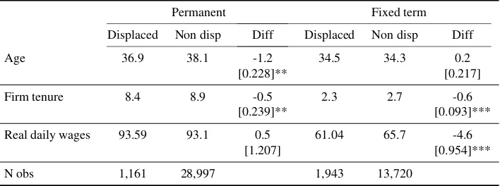
Tables 1.1 to 1.3 present sample characteristics of displaced workers during mass-layoffs. These tables show that there are important differences between displaced and non displaced, and under the two types of contracts. Table 1.1 shows differences in workers characteristics in 1997 (the beginning of the sample), that is pre-treatment pe-riod. First, displaced workers under PC tend to be younger than non-displaced PC work-ers, while for FTC workers the difference is not significant. On the other hand, displaced workers tend to have shorter firm tenure. Displaced from fixed term contracts tend show lower wages than the non-displaced counterpart, but for the PC workers this difference is not significant. These differences are also present between the two type of contract.
3
That is, fixed term workers are younger, lowered tenured and earn lower wages, than their open-ended contracts counterparts.
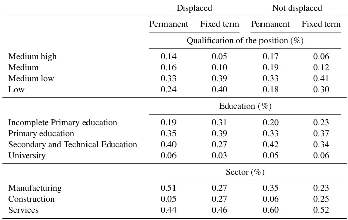
As table 1.2 shows, displaced workers tend to be lowly educated and occupy posi-tions that require lower qualification (second panel of the table). These differences are also present when comparing PC and FTC workers. Fixed term workers tend to be lower educated, and occupy lower qualification positions, than the PC counterparts. Finally, as the third panel of that table shows, PC workers suffer mass-layoff mainly from manu-facturing and service sectors, while for FTC workers, the construction sector is also very important.
These pre-separation differences highlight the importance of controlling for observ-able and unobservobserv-able characteristics of the displaced workers when comparing them to a control group, something that is going to be address in the regression analysis.
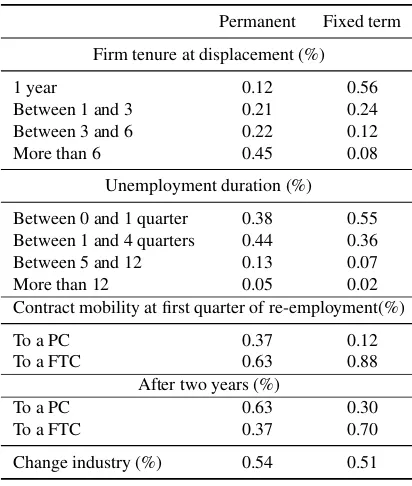
Finally, table 1.3 shows differences in the displacement event between temporary and permanent workers. First, firm tenure at displacement is much shorter for fixed term workers4. Second, workers displaced from permanent contracts tend to experi-ence longer unemployment spells. Third, more than 60% of workers holding indefinite contracts at displacement are re-employed with fixed term contracts5. This figure is larger for workers holding fixed term contracts at displacement (almost 90%). Hence, displaced workers enter a mobile market with high incidence of temporary contracts. After two years of being re-employed, PCs workers tend to have more probability of re-gaining a PC while most FTCs still mantain the temporary status. Finally, almost half of these workers change industry after displacement. The industries are measured at two digit level. The figures are similar between the two type of workers, showing that changing industry is not more probable for any of the two contract arrangements after a mass-layoff event.
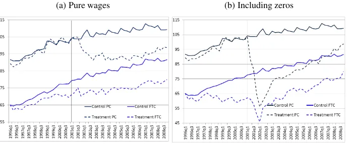
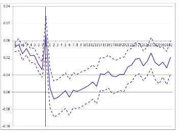
Figures 1.1a and 1.1b show the daily real wage path of individuals who separate from employment in 2001 relative to the control group. Figure 1.1b shows the wage path including the periods of unemployment with zero wages, while figure 1.1a shows only pure wage effects, i.e. being missing observations when unemployed. It is notable that before separation wages trends are similar relative to each other, for both types of workers. Figure 1.1a is the most interesting for us, since the regression analysis will have as dependent variable the logarithm of wages. If anything, there appears to be a simple intercept difference in the starting point of the wage paths at the start of the sample period between displaced and non-displaced, and permanent and fixed term con-tracts. Thus, estimators such as the fixed-effects, which control for individual specific
4
Most of fixed term contracts may not be extended after 3 years, although changing the nature of the job for hiring the same worker under subsequent temporary contracts has been a common practice among Spanish employers. This and the fact that “per task or service” contracts are easily extended, explains the high tenures of some fixed term employees.
5
intercepts would be expected to effectively equalize earnings prior to job separation. Ad-ditionally, the figures show that workers experienced substantial long-term wage losses. The earning losses in figure 1.1b are larger than in figure 1.1a, related to the zero in-come during unemployment. In figure 1.1a, where pure wage losses can be analyzed, we can already see that fixed term workers experience much lower wage losses, if any, than workers holding permanent workers at the time of displacement.
1.3.3
Methodology
A key lesson from the literature is that is not sufficient to measure wage losses as the difference between workers’ earnings in some post-displacement period and their earn-ings in a period shortly before separation. Some reasons why this measure may not capture the full effect of displacement on workers’ earnings are: it does not control for macroeconomic factors that cause changes in workers’ earnings regardless of whether they are displaced; does not account for the earnings growth that would have occurred in the absence of job loss; and, firms’ declining fortunes may adversely affect workers’ earnings several years prior to their job loss, as Jacobson et al. (1993) argued. Thus, the displaced workers’ wage losses are defined as the difference between their actual and counterfactual wage that would be prevalent if the events leading to separation had not occurred.
The idea is to compare wages of non displaced versus displaced workers. An aug-mented mincerian wage equation that captures the difference in earnings across dis-placed and non-disdis-placed workers, can be estimated:
yit=αi+µt+βXit+
X k
γkDkit+ X
k
δkDkit∗P C 0
i +ηP Cit+εit (1.1)
yitis the logarithm of the real daily wage earnings for individual i at period t. Wages were deflated by the CPI (base: January 2008). The displacements episodes are repre-sented trough a set dummy variables:Dk. These dummies are equal to one if individual
con-tract hold at every tP Cit, whereηcaptures any premium in wages between permanent and fixed term workers, after controlling for observed and unobserved characteristics.
µt are time effects that capture the general time pattern of earnings in the econ-omy.αisummarizes permanent differences among workers in observed and unobserved characteristics. The error termεitis assumed to have constant variance, and to be un-correlated across time and individuals.
This strategy is a form of the differences-in-differences (DiD) estimation method, which in this case is implemented by using a fixed-effects estimator. Much of the litera-ture on displacement recognizes that the event is likely to be non-random. Non-random assignment is likely to be a problem, even for a mass-layoff or plant-closings sample. Employer selection suggests that those workers with lower productivity will be displaced in a mass-layoff, while employee selection suggests that those workers whose outside job prospects are better will choose to leave. In the case of firm closure, it may be that those workers who remain in the firm until closure are a non-random sample of all those in the firm at the point where closure become public knowledge.
If selection into the treatment and control groups is on the basis of permanent char-acteristics embodied in workers’ fixed effects and the observable charchar-acteristics, then equation 1.1 will yield consistent estimates of the expected wage loss. Hence, the as-sumption for interpretingγkandδkas causal impact of job separation is that conditional on fixed effects and included observable characteristics, displaced workers are observa-tionally equal to the workers in the control group. In any case, Appendix 1.9 shows a robustness checks including specific time trends.
Another comment we need to make at this point, is that estimations are only taking into account people that find jobs again. There can be a problem in selection since we only observe successful people that manage to be re-employed again. Since, the idea of the study is to analyze pure wage effects of job displacement in order to capture the implication of the human capital theory, we restrict to this case.
1.4
Empirical results
1.4.1
Wage losses after displacement
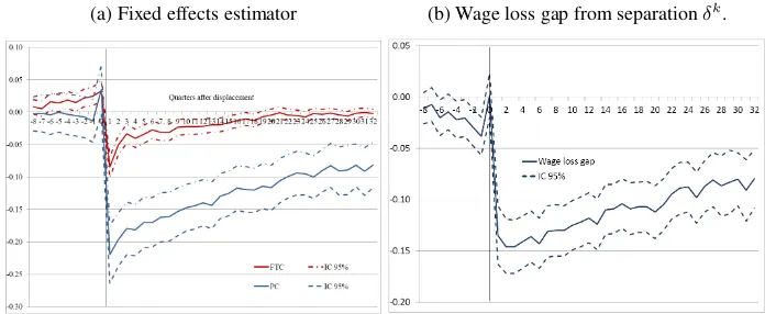
to the control group. 6 In the fourth year following displacement, substantial recovery occurs and the estimated impact average 11,7 percent. The estimated wage losses for workers holding FTCs at the time of displacement are much lower. The first quarter after displacement suffer an 8,5 percent wage losses relative to the control group, while after four years of displacement, substantial recovery occurs and the estimated impacts average 1,3 percent, being not statiscally significant.
As shown in figure 1.2b the differences in the wage losses between displaced from permanent or fixed term contracts are always significant, indicating that permanent con-tract workers loss more wages after a mass-layoff than their fixed term counterparts. The gap is 15% in the first quarter after displacement, recovering slowly till 10% 6 years af-ter.
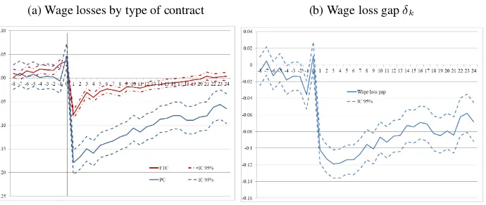
One of the main reasons behind the differences in the wage losses after displacement between PC and FTC is the clear differences in firm tenure that arise from table 1.3. In order to see if these differences are still present when restricting by tenure, we are going to apply the same methodology but taking into account, both in the control and treatment group, workers with less than three years of tenure in the last quarter of 1998, i.e. the quarter before I allow for mass-layoffs to happen.
Figure 1.3a shows the graphical representation of the coefficients in equation 1.1 using only workers with less than three years tenure. Results are robust. The figure is very similar to figure 1.2a, but now the point estimates for PC workers are lower. This makes sense since we are restricting to people with lower tenure, and hence lower accu-mulation of specific human capital. The wage loss gap, in figure 1.3b, is 10% in the first quarter after displacement, and four years later still remains very high (7%).
Appendix 1.9 shows some robustness checks including specific time trends, and es-timating the wage losses depending on the type of contract the worker has been able to obtain after two years of being re-hired.
1.4.2
Decomposition of wage losses
According to Becker’s theory, if job tenure contributes to the accumulation of specific human capital or seniority rights, it should be positively associated with wage losses. On the other hand if, a component of wage gains are due to industry-specific capital, then displacement should affect future wages only in the event that workers switch industries. Finally, if deterioration of general human capital during unemployment happens, or an unemployment spell serves as a signal of low productivity, wage losses should increase with the duration of unemployment.
6
This exercise shows the decomposition of the wage losses in different sources, using equation 1.1 :
1. loss that stems from the loss of job tenure→firm specific skills, or seniority
2. loss related to changing industry→loss of sector specific skills
3. loss associated with unemployment duration→depreciation of general human capital, or signal of low productivity
The idea is to include to the baseline equation, one by one possible determinants of the wage losses. Including these variables we are explaining the wage losses, hence the es-timated losses are the wage losses that remain after controlling for these sources. Thus, we expect a decrease in the estimated coefficients (δkandγk).
First, I am going to compute how the wage losses change when including the pos-sible determinants, i.e. the coefficients on the displacement dummies, at one year after displacement,k = 4. After including each determinant, we are going to impute the change in the wage losses (the estimated coefficients) to that variable (e.g. unemploy-ment duration). Since the estimated coefficients are sensible to the order on how we include these determinants, I am also going to change the order how these variables are included, and calculate the maximum and minimum change of the wage losses. These are interpreted as the range of change of the wage losses due to the different determi-nants.
The possible determinants included are pre-displacement tenure (equal to the tenure in the firm where the worker suffered the mass-layoff), duration of unemployment (total duration of unemployment after the mass-layoff), and a dummy variable that is equal to one after the mass-layoff if changed industry at two digit level in the new job. These variables are equal to zero before displacement and for the control group. This is like multiplying a dummy equal to one after displacement, by unemployment duration, pre-displacement tenure or if change industry. At the same time, these variables are in-teracted withP C0, the dummy that indicates if the worker had a PC at the time of displacement, in order to analyze the effects by type of contract.
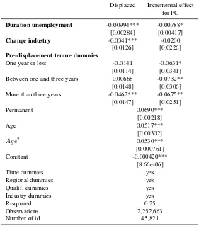
First, the analysis of the coefficients on the determinants is performed. Table 1.4 shows the the regression estimates after including all the determinants explained above. On average, one quarter of duration of unemployment rises the losses in wages, relative to the control group, in 0.99 percentage points (p.p.) for workers displaced from FTC, while 1.77 p.p for PC workers. This difference is statically significant, showing that duration of unemployment has a larger negative impact on worker displaced from PC.
Finally, dummies for pre-displacement job tenure have been included. Having less than three years of pre-displacement tenure has no significant effect on post-displacement wages of FTC. The impact is negative and significant for worker with more then three years tenure under FTC, increasing the losses in 4.6 p.p.. For permanent contract work-ers, pre-displacement tenure has negative impact on wage losses after displacement, and increases with pre-displacement tenure. For workers with a year or less of tenure in the displacement job wage losses increase by 6.3 p.p.. For workers with tenure between one and three year this reaches to 7.3 pp and for more then three years 11.4 pp. This differences with respect to FTC workers are significant. This is evidence of different accumulation of job specific capital human capital between the two type of contracts, supporting the prediction of the human capital theory.
We can now turn to analyze what happens with the displacement dummies for the two type of workers. After including the determinants, the estimated wage losses can be interpreted as if workers did not experience unemployment, did not change industry, and did not loss tenure. Table 1.5 shows the change in the coefficients on the displacement dummy after a year of displacement in the base line equation 1.1. Since, the estimated coefficients can be altered by the order of inclusion of these determinants, the table shows the maximum and minimum of the change in the wage losses depending on the order.
As shown in the table 1.5, pre-displacement tenure is the more important source for explaining wage losses of PC workers; between 25% and 50% of their losses are ex-plained by the loss of pre-displacement firm tenure, while between -20 and 20% of FTC losses, showing that is not significant. Again, this is evidence of the difference in the investment of firm specific human capital between the two type of contracts, confirming the hypothesis of lower investment in FTC. Controlling for unemployment duration is important to explain FTC and PC wage losses. From 6 to 22%, and from 14 to 23% of the wage losses of FTC and PC, respectively, are explained by the time spent in unem-ployment. Finally, the losses from changing industry explain a lower share of the wage losses, even if it seems to be very sensitive to the order on how we include variables. In any case, this is evidence that even if the accumulation of industry specific capital is important, is not different between the two type of contract arrangements.
1.5
A model of dual labor markets and firm specific
hu-man capital
This section presents the model, an extension of the canonical search and matching model with endogenous separations (Mortensen and Pissarides (1994)), that allows for the existence of permanent and fixed term contracts.
The economy consists of a continuum of risk-neutral, infinitely-lived workers and firms. We normalize the measure of workers to 1. Workers and firms discount future payoffs at a common rateβ. Moreover, capital markets are perfect and time is discrete. Workers may be either unemployed or employed. Unemployed individuals enjoy an in-stantaneous utilitybeach period. Those who are employed can be so either under a fixed term or a permanent contract.
Firms decide which type of contract to offer when matched to the workers, and de-cide when to endogenously separate, or promote the worker to a permanent contract (PC). Separating endogenously from a worker holding a permanent contract entails an exogenous costF, while separating from a fixed term contract (FTC) is costless. This way, F reflects the firing cost gap between the two type of contracts. Exogenous separa-tions may also occur at no cost with probabilityδfor any type of worker. When the pair separates, endogenously or exogenously, the worker becomes unemployed.
Moreover, fixed term contracts expire each period with probabilityλ. This param-eter can be interpreted as the inverse of the mean duration of this contracts. The higher
λ, the lower duration of FTCs. This parameter reflects legal restrictions regarding the use of fixed-term contracts, such as the limited number of renewals and the maximum duration of the contracts. A higherλ, in this model, indicates stringer legal restrictions in the use of FTC. At expiration, the firm decides if separate from the worker, or keep the worker and promote her to a permanent contract. Thus, while the expiration rate is constant the conversion probability is an endogenous variable in the model.
The dual economy is going to be defined by two policy parameters: the firing costs gap in permanent contracts,F; and the expiration rate,λ. At expiration firms decide if promote the worker and give a PC, or lay-off the worker. Firing costs in this model are not severance payments. Severance payments are a transfer from the firm to the worker, do not entail any difference in these type of models; unless other rigidities are added, such as minimum wages. The firing costs,F, are paid by the firm in case of separation, and are consider a waste. They can be interpreted as red tape costs, costs of judge for laying off a worker, etc.
Workers decide if invest in firm specific human capital (FSHC)7. Investing in FSHC entails a cost,C, and instead the workers become immediately more productive by an
7
amounts. As a simplifying assumption, the investment is made at the moment of real-ization of the contract, and the worker becomes immediately more productive. Note that since the acquired human capital is firm-specific, it is completely lost upon displace-ment.
Each firm consists of only one job which is either filled or vacant, and uses only labor as input. If the vacancy is filled, it producesεt, the idiosyncratic productivity of the match, which has a cumulative distribution functionG(ε), independent and identi-cally distributed across firms and time, and is assumed to be log-normal. Thus, shocks to this idiosyncratic productivity happen every period. No persistence is assumed in this model.
Unemployed and vacancies meet according to a standard matching function with constant returns to scale: m(u, v) = ψuv1−α. Labor market tightness is defined, as standard in the literature, as the ratioθ=v/u, and the probability that an unemployed worker meets a vacant job is defined asp(θ) = m(u,v)u , and the that a vacancy meets a worker isq(θ) =m(u,v)v .p(θ)is increasing inθ, whilep(θ)is decreasing.
After a match is realized, a match specific productivity is drawn. If the match is profitable the firm hires the worker. Workers and firms bargain over wages according to standard Nash bargaining every period. Finally, there is free entry, i.e. firms open vacancies until the value of a vacancy is driven to zero.
The timing of the model is the following. At the beginning of each period unem-ployed workers and vacancies meet. At the same time, all existing matches (i.e., those who produced last period) learn whether they break exogenously with probability δ. Right after that, surviving temporary matches realize whether their contracts expire ac-cording to probabilityλ. Afterwards, each match (old and new) draws an idiosyncratic productivityε.
Then, workers decide if invest, correctly anticipating the type of contract to be of-fered, duration of the job and the result from the wage bargaining. Firms decide the type of contract to offer, and bargain an entry wage, and after every productivity shock bargain again. PC contracts are protected from separation by firing costs, after the first period, which is paid by the firm in case of separation. At the same time, if FTC expired the firm decides if convert it to a PC or lay-off the worker.
Note that, the assumption is that investment is non-contractible or unenforceable. Due to the nature of specific investments, training or the effort to become more pro-ductive cannot be contracted. The cost of investment is sunk before reaching the wage bargaining. Hence, it can be interpreted as the effort workers need to do to be trained which is not observable by firms.
From now on, the steady state properties of the model will be analyzed. Hence, we can abstract from aggregate productivity shocks.
1.5.1
Match surplus and wage bargaining
The firms’ value of fixed term or temporary and permanent contracts is defined asJT(ε)
andJP(ε), respectively. While, the workers’ value of temporary and permanent jobs is defined asWT(ε)andWP(ε)8. The values of unemployed and vacant jobs are U and V, respectively9.
Since temporary contracts separate costlessly, the total surplus of a match will be
ST(ε) =JT(ε)−V +WT(ε)−U
However, when a permanent match separates the firm has to pay the firing costF, lowering its outside option toV −F. Therefore the total surplus is:
SP(ε) =JP(ε)−V +F+WP(ε)−U
The first period of a permanent contract does not entail this firing cost, since if there is no agreement on the contract, the firm is not liable to pay the firing cost. The firms’ and workers’ value of permanent contracts in this initial period are defined asJP
0(ε)and
W0P(ε). Hence, the the surplus can be written as:
S0P(ε) =J0P(ε)−V +W0P(ε)−U
Wages are determined by Nash Bargaining between firms and workers every period, as a new draw from the idiosyncratic productivity arrives. Hence, the sharing equations hold every period. The workers’ bargaining power is defined asφ, hence the surplus-sharing rules are:
ST(ε) = (1−φ)(JT(ε)−V) =φ(WT(ε)−U) (1.2)
SP(ε) = (1−φ)(JP(ε)−V +F) =φ(WP(ε)−U) (1.3)
S0P(ε) = (1−φ)(J0P(ε)−V) =φ(W0P(ε)−U) (1.4) And the wage functions:wT,wP, andwP
0.
1.5.2
Job creation and job destruction
The value of a filled vacancy is showed in equation 1.5. Firms post vacancies with a cost flow ofa. When matched to a worker decide which type of contract to give the worker,
8
Remember here we abstract from aggregate productivity shocks, and here the firms and work-ers value only depend on the idiosyncratic productivity of the match
9
maximizing the value of a filled vacancy under the two type of contracts. We can discuss three cases, one in which workers invest in FSHC in both contracts, one in which only invest in FTC, and one in which only invest in PC.
Vt=−a+β[q(θt) Z ∞
0
max
Jt+1T i (z), J0,t+1P i (z),0 dG(z) + (1−q(θt))Vt+1] (1.5)
wherei=I, N I.
The first case is if both contracts I (invest) or NI (not invest) in FSHC. Considering all future realizations ofε, the expected income flow from temporary and permanent contracts is the same every period until separation. The difference is that upon displace-ment the pair in a PC lossesF, henceWP+JP < WT+JT. At the same time, offering a PC lowers the firms’ threat point from 0 to−F. Hence, since offering a PC diminishes the joint payoff, and lowers the firms’ threat point, a firm will always prefer to offer a FTC if legally allowed to do so.
Second, the case FTC workers invest in FSHC but PC do not. According to the re-cent argument, firms will always offer a FTC. Even more in this case, in which PC will have a lower income flow than FTC workers, and lower threat point and the firing costs in case of displacement.
In the third case, PC workers invest in FSHC, while FTCs do not. In this case, the expected income flow from permanent contracts is larger than for fixed term contracts, bys, the productivity gain of inventing in FSHC. But still at separation the pair losses
F, and firms’ threat is reduced from zero to−F. Hence, the decision is going to depend on the relative size of the productivity gain due to the investment,s, and the firing costs,
F. If the productivity gain is not much larger than the separation costs, the firm will still offer a temporary contract when matched to a worker. In fact, this true for a wide range of parameters; even more when analyzing the Spanish economy where firing costs are large. Hence, I restrict to study this case10.
Hence, if a firm is legally allowed to hire under fixed term contracts, it will always choose to offer the worker a fixed term contract over a permanent contract.
There is free entry of firms in the economy, hence firms post vacancies until the point the value of a vacancy is zero:V = 0. Job creation and separation will be determined by three productivity thresholds, above which production takes place or continues. The first is the threshold for hiring and firing temporary contracts:εT, such that any eligible job continues ifεt> εT. This threshold is defined as the match productivity that makes the firms value equal to zero, wherei=I, N I:
JT i(εT i) =ST i(εT i) = 0 (1.6)
10
Second, there is the promotion threshold, that is relevant when the FTC expires,εP0, such that any job no more eligible from FTC is converted to a PC ifε >P
0. At this point the firm is indifferent between converting to a permanent contract or separating costless. The threshold is determine by
J0P i(εP i0 ) = 0⇒S0P i(εP i0 ) = 0 (1.7) Finally, the threshold for firing permanent contracts isεP, and is determined by:
JP i(εP i) +F = 0⇒SP i(εP i) = 0 (1.8)
From all above, it can establish an ordering of the thresholds from this economy. From equations 1.8 and 1.7 we can establish thatεP i0 =εP i+F. On the other hand, as stated above firms always offer worker FTC instead of PC when matched to a worker. This implies that FTC is the preferred option for firms. At expiration, the firms choice set is shrank, eliminating the preferred choice, and this match is less valuable, which implies that the threshold for firing and hiring FTCs is above promotion threshold (which is the same as hiring threshold for PC):εT < εP
0. Finally, given the firing costs in PC, the threshold for firing PC lies bellow the one for FTC. We already now that firms prefer to offer a FTC than a PC: WP +JP < WT +JT, but PC matches do not separate unless the surplus goes bellowF. Therefore,WP +JP +F > WT +JT, implying
thatεP < εT. This means that matches under PC accept lower productivity just to avoid
payingF. Thus, the firing threshold for PC lies below the firing threshold for FTC, which lies below the promotion threshold.
Hence,
εP i< εT i< εP i0 (1.9)
At the same time we know that if the worker invests the threshold is lower than if the worker does not invest. This reflects the fact that if the worker invests the separation rate is lower. Hence,
εjI < εjN I (1.10)
wherej=T, P
In the appendix 1.10 can be found the rest of the detailed surplus functions for tem-porary and permanent contracts, as well as the steady state equilibrium conditions and steady state employment and unemployment.
1.5.3
The workers’ decision of investment in firm specific human
capital
workers’ value of a job knowing that the investment entails a cost C, so that:
max
WjI(y)−C, WjN I(y) (1.11) wherej=T, P temporary or permanent contract.
When matched to a firm, the workers know he is going to be offered a temporary contract. In the equation 1.12, the value of unemployment, the maximization problem can be seen. The value of unemployment is equal to the income flow of being unem-ployed,b, plus the discounted expected future income. The moment they get hired pay C if invest, lowering the value of unemployment, but become immediately more produc-tive, bys.
U =b+β[p(θ)
Z ∞
0
max
WT I−C, WT N I, U + (1−p(θ))U] (1.12)
After some algebra we can write the condition under which FTC workers invest de-pending on the threshold of firing temporary workers in equation 1.13.
φ(εT N I−εT I
| {z }
>0
) + ∆U−C≥0 (1.13)
This condition has three parts. The first, is the difference in the firing thresholds un-der temporary contracts. As shown is equation 1.10 this difference is positive reflecting the lower separation rates if workers invest in FSHC. The second part reflects the change in the unemployment value. This change is negative because investing lowers the value of unemployment. Finally, the cost of investment. Hence, the investment decision will depend on which of the these trade-offs domains. Note also, that the largerφ, the work-ers’ bargaining power, the higher the likelihood of investment. While the lower cost of investment,C, the higher likelihood of investment.
The decision problem for PC workers is very similar. In this case, if the FTC ex-pires workers decide if invest in FSHC under PC. Hence, they are going to maximize the value of employment under permanent contracts at the time of promotion. Equation 1.14 shows the value of employment for a temporary contract, where this decision is embed-ded .
WtT i = wtT i+β
(1−δ)
(1−λ)
Z
0
maxWt+1T i(s), Ut+1
dG(s) +
+ λ
Z
0
max
Wt+1,0P I (s)−C, Wt+1,0P N I(s), Ut+1
dG(s) + δUt+1
The workers’ value of a temporary job is equal to the income flow, i.e. the wage, plus the expected income. If not exogenously separated and the contract does not expire, the value for a worker of a temporary job provided that the new idiosyncratic shock is above the threshold. In the case of expiration of contract, provided that the idiosyncratic productivity is above the promotion threshold, the value for the worker of a permanent job. If the worker decides to invest need to pay the costC.
This maximization problem can be re-written as:
φ(εP N I−εP I
| {z }
>0
) + ∆U −C≥0 (1.16)
As in the case for temporary contracts, this condition has three parts. The first is related to the fact that after investment the threshold for firing in permanent contracts is lower (also the threshold for promotion). And the second and third part are related to the fact they have to pay the cost C, which changes the workers’ value of employment of a temporary worker, and hence the unemployment value. Again, the decision of in-vestment depends on the relative size of these effects on the threshold and the cost of investment,C.
The conditions for investment in temporary contracts, equation 1.13, and permanent contracts, equation 1.16, depend on the parameters of the model. More specifically on policy parameters that determine the duality of the economy:F, andλ. The next step is calibrating the model to then show how these parameters affect the decision of workers.
1.5.4
Wage losses in the model
As shown in the empirical work, I found evidence of a gap in the invest in FSHC, in which PC workers invest more than FTC, that translates in to a wage loss gap of 6% in the first quarter after displacement. Hence the strategy is calibrating the model assum-ing that PC invest, but FTC does not invest. This way the gain in productivity,s, can be interpreted as the produtivity gap due to the investment gap in firm specific skills. To be more clear, the wage equations are described in the following equations in the case PC workers invest and FTC workers do not:
The wage loss is defined with respect to the entry wages: wT, hence FTC workers show zero wage losses.
χT =E(wT N I)−E(wT N I) = 0
While PC workers are going to be displaced from PC, and re-hired under a FTC, hence losing all the investment in FSHC.
χP = E(wP I)−E(wT N I) =φ
E(ε/ε > εP)−E(ε/ε > εT) +
+s+F(1−β(1−δ))−(1−φ)β(1−δ)λ(1−G(εP I0 ))C
(1.18)
As argued in the empirical analysis, the gap found is due to the investment in FSHC, since we control for other premiums in wages, and other sources of wage losses. Hence, we can calibrate the wage loss gap found due to the difference in FSHC as:
χP =φs (1.19)
1.6
Calibration and results
1.6.1
Calibration
The calibration of the model is done at quarterly frequency in order to match four targets that characterize the Spanish economy. The baseline parametrization is summarized in Table 1.6.
The first three parameters in the table are taken from the standard literature of search and matching, setting the quarterly discount rateβto 0.99. Then I choose other param-eters following literature for Spain. Petrongolo and Pissarides (2001) indicate that the elasticity of the matching function is in between 0.5 and 0.7. We set it at 0.5 as Costain et al. (2010) and Bentolila et al. (2010). As standard in the literature, it is assumed that workers’ bargaining power is equal to the elasticity of the matching functionφ=η. As in Costain et al. (2010) the unemployment income flow,b, is set relative to the steady state equilibrium cross-sectional average worker productivity,Eε, and equal to 0.8. Usu-ally, for US is used a parameter of 0.7, but since in Spain the unemployment benefits are higher, instead set b to a larger amount. The cost of posting vacancies,a, is set to 0.3 which the mid-point found in the literature11. Following also Costain et al. (2010) we set
the exogenous probability of separation to 0.00625, which implies a worker who does not experience endogenous separations, stays in the same job a mean for 40 years.
As standard in the literature, I normalize the mean of the underlying log productiv-ity distributionµ=E(log(ε))to 0, while the standard deviation is chosen to match the share of temporary workers in the Spanish economy, i.e. nnT = 0.3. The expiration rate of FTC, a policy parameter, is set to last a mean of two years and a half,λ= 1/(30/3)12. The exercise has four targets, the share of temporary workers in the Spanish econ-omy, the outflow rate from unemployment, the inflow rate from unemployment for per-manent contracts, and the conversion rate from fixed term to perper-manent contracts. The job finding rate is taken from Elsby et al. (2013) who calculates monthly outflows and inflows rates from unemployment for OECD countries using data on duration of un-employment. The job separation rate of PC is calculated using data from Silva and Vázquez-Grenno (2012) who calculate quarterly transition probabilities in the Spanish labor market using the data from the Spanish Labor Force Survey (SLFS), taken into ac-count that employment is divided between permanent contract jobs and temporary jobs. They calculate these rates from a three state set up (employment, unemployment and inactivity). Since in the model unemployment and inactivity are the same, we take both into account. The average rates are calculated over the period 1995 to 2007.
The separation rate from permanent contracts is used to set the firings costsF, while the job finding rate is targeted to calibrate the parameter of efficiency in the matching function. Finally, the conversion rate is used to obtain the cost of investment in FSHC for PC,C.
Finally, I match the gain in productivity to a 6% wage loss gap. According to equa-tion 1.19 and the value for the workers’ bargaining power, this implies a gain in pro-ductivity for PC workers of 12% due to the investment in firm specific human capital. This seem to be a resonable parametrization. Sala and Silva (2009) calibrate their model to Spain with a productivity gap between permanent and fixed term contracts of 20%. They base their estimates in Aguirregabiria and Alonso-Borrego (2004), who estimate the productivity of a temporary worker to be on average 80% of the productivity of a permanent worker. This model is implying a lower productivity gap.
1.6.2
The investment decision
In this subsection the conditions for investment in FSHC of FTC workers in equa-tion 1.13, and of PC workers in equaequa-tion 1.16 are analyzed. The first goal is to cor-roborate that PC workers want to invest, and FTC workers do not. The second goal is
12
to understand how these conditions depend on the policy parameters that determine the duality of the economy:Fandλ.
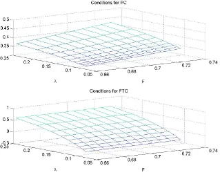
The next figure shows how the conditions in equation 1.16 (above panel), and equa-tion 1.13 (bellow panel) change with the policy parameters. The graph shows the con-ditions for investment when changingF by±5%, and λ1 from to 4 quarters (λ= 0.25) to 3 years (λ= 0.83). The picture can be interpreted as the likelihood of investment. If it has positive sign workers want to invest in FSHC, while if negative worker will not invest. Note that in this simple model, the investment is done in a fixed amount, hence, the larger is this condition, the larger is the likelihood of investment, but not the larger investment.
First, we can see that PC workers always want to invest under this calibration, since this condition is positive for all the combination of parameters shown. As we can see from the graph this condition is increasing inF andλ. It can be shown that ∂ε∂FP <0, the higher the firing costs, the lower separation rates from PC, i.e. longer duration of the job. This cut-off increases more if PC workers have invested, increasing the likelihood of investing in PC. At the same time,∂ε∂λP <0, thus the higher the expiration rate (lower duration of contracts), the lower separation rates in PC, meaning that firms are less se-lective to convert into PC, and to layoff PCs. This cut-off decreases more if PC workers have invested, increasing the likelihood of investing in PC. This is because firms become less selective in PCs in general, and can rely less in FTC. Since FTCs expire faster, and firms have to look for other workers, which is costly, they becoming less selective.
On the other hand, the condition for investment for FTC workers in the baseline calibration is negative, and only becomes positive for higher values ofλ. The condition is also sightly increasing inF. This suggests that FTC workers would only invest for high values ofλ, andF. It can be shown that ∂ε∂λT > 0, the larger the expiration rate (lower duration of contracts), makes firms more selective to hire FTC, but less if FTC invests, increasing the likelihood of investment in this type of contract. Also, ∂εP0
∂λ <0, meaning an increasing conversion rate withλ. It increases more if FTC invests in FSHC, increasing the likelihood of investing in FTC. Finally, ∂ε∂FT >0. The higher the firing costs, the higher separation rates from FTC. This is the other side of sclerosis in PC, increasing the churning for FTC. This cut-off increases less withFif FTC had invested, increasing the likelihood of investing in FTC. In any case, as the picture shows under this parametrization the condition of investing for FTC remains almost constant with F, not affecting FTC contracts.