Essays on New Keynesian Macroeconomics
José Antonio Dorich Doig
Address: Llacuna 142 5-3, Barcelona, Spain
Email: [email protected]
Phone: 649725641
Dissertation submitted for the degree of
Doctor of Philosophy
in Economics
Acknowledgements
I would like to express my gratitude to all the people who made this thesis possible. I am deeply indebted to my supervisor Jordi Galí. Throughout my doctoral studies, he provided excellent guidance, sound advice, great teaching, and excellent ideas. It was really a pleasure and an honor for me to have had the possibility of discussing my research with him. I am also very indebted to Thijs van Rens for his encouragement and excellent academic support. I received invaluable comments from him.
The research that I present in this thesis also bene…ted from many comments and discussions with Filippo Brutti, Andrea Caggese, Fabio Canova, Davide Debortoli, Francisco Grippa, Albert Marcet, Ricardo Nunes, and Michael Reiter.
I am also very grateful to Marta Aragay, Marta Araque, Gemma Burballa, Anna Cano, Carolina Rojas, and Anna Ventura. They kindly assisted me with all the ad-ministrative issues related to my doctoral studies.
Contents
Introduction 1
1 The Welfare Losses of Price Rigidities 5
1.1 Introduction . . . 5
1.2 The Model . . . 7
1.2.1 Households . . . 8
1.2.2 Firms . . . 9
1.2.3 Equilibrium . . . 10
1.3 The Welfare Losses of Price Rigidities . . . 10
1.3.1 A Second Order Approximation to Utility . . . 11
1.3.2 An Analytical Expression for the Welfare Losses . . . 11
1.4 The Welfare Losses with Calvo Pricing . . . 13
1.4.1 Calvo Price-Setting . . . 14
1.4.2 Measuring Welfare Losses . . . 17
1.4.3 Quantifying LIPt . . . 18
1.5 Welfare Losses with State-Dependent Pricing . . . 25
1.5.1 The Model . . . 25
1.5.2 Measuring Welfare Losses . . . 27
1.5.3 Quantifying V arifxt(i)g . . . 28
1.6 Concluding Remarks . . . 32
2 Testing for Rule of Thumb Price-Setting 33 2.1 Introduction . . . 33
2.2 The New Keynesian Hybrid Model . . . 35
2.2.1 Households . . . 36
2.2.3 Aggregate Price Level Dynamics . . . 37
2.2.4 The Hybrid NKPC . . . 37
2.3 Relationship Between the Cross Sectional Variance of Individual Price Changes and Aggregate In‡ation . . . 39
2.4 Empirical Evidence . . . 40
2.4.1 Econometric Speci…cation . . . 40
2.4.2 Data and Estimates . . . 41
2.5 Comparison with Galí and Gertler (1999) . . . 42
2.6 Concluding Remarks . . . 44
3 Resurrecting the Role of Real Money Balance E¤ects 47 3.1 Introduction . . . 47
3.2 Money in Utility Function Model . . . 49
3.3 New Estimates of Real Money Balance E¤ects . . . 52
3.3.1 Econometric Speci…cation . . . 53
3.3.2 Data and Baseline Estimates . . . 55
3.3.3 Robustness Exercises . . . 58
3.3.4 Previous Studies on Real Money Balance E¤ects: a comparison 63 3.4 Implications of my Findings . . . 66
3.4.1 MIU Model with Monopolistic Competition, Sticky Prices and Flexible Wages . . . 67
3.4.2 The Modestly Procyclical Real Wage Response to a Monetary Policy Shock . . . 70
3.4.3 The Supply Side E¤ects of Monetary Policy . . . 72
3.4.4 The Impact of Real Money Balance E¤ects on the Design of Optimal Monetary Policy . . . 73
3.4.5 The Diminishment in the Size of Real Money Balance E¤ects, Greater Macroeconomic Stability and Financial Innovation . . . 75
3.5 Concluding Remarks . . . 78
A Addendum to Chapter 1 81 A.1 The Adjusted Output Dispersion (dt) . . . 81
A.2 The Relationship between dt dnt and the Dispersion of Price Gaps Across Goods . . . 83
Introduction
The standard New Keynesian (NK) model has become one of the most in‡uential tools in discussions of macroeconomic dynamics, monetary policy and welfare. Moreover, it has emerged as the backbone of the medium scale macroeconomic models that several central banks and policy institutions use for simulation and forecasting purposes. This model integrates the Real Business Cycle (RBC) Paradigm with NK Theory. In fact, the NK model adopts a stochastic dynamic general equilibrium modeling approach from the RBC theory and combines it with two Keynesian ingredients: monopolistic competition and nominal price rigidity. In this sense, this model has much stronger theoretical foundations than traditional Keynesian models.
The purpose of this thesis is to evaluate the accuracy of the following three impli-cations of the standard NK model. First, with full price stability the welfare losses resulting from price stickiness should be zero. Second, in‡ation is a forward-looking phenomenon. Third, money does not play an independent role in the monetary trans-mission mechanism.
Traditionally, price stickiness has been studied within the New Keynesian frame-work as a source of monetary policy non-neutrality or to understand in‡ation persis-tence. In contrast, I try to answer the following question in this thesis: how harmful can price stickiness be for society? Theoretically, in the face of exogenous shocks, this rigidity can cause welfare losses by creating relative price distortions that lead to an ine¢ cient sectoral allocation of resources. According to the standard NK model, by attaining zero in‡ation, relative price distortions are eliminated and the economy reaches the ‡exible price allocation.1 Therefore, in the NK setup, monetary policy is able to avoid all the welfare losses that could arise from price stickiness.
In chapter 1, titled "The Welfare Losses of Price Rigidities", I introduce
speci…c productivity shocks in the standard NK model and compute the welfare losses of price stickiness. Moreover, I also depart from the time-dependent pricing assump-tion that is used in the NK model. In particular, I compute the welfare losses when price rigidities are incorporated by using state-dependent pricing.2 Several interest-ing results stand out. First, price stickiness may be a source of large welfare losses, even in economies with price stability. Second, state-dependent pricing dampens the size of the welfare losses, but they remain non-negligible. Third, the variance of the …rm-speci…c productivity shock and the frequency of price adjustment are the key determinants of the size of the welfare losses.
Studying in‡ation dynamics is crucial for monetary policy analysis; in particular, exploring how plausible it is that in‡ation is mainly determined by forward-looking behavior. This is especially important for understanding the di¤erent sources of in‡a-tion persistence and the costs of disin‡ain‡a-tion processes.3 The New Keynesian Phillips Curve (NKPC), which describes the aggregate supply block of the NK model, predicts that in‡ation is determined exclusively by forward-looking behavior of …rms. However, several studies have found evidence of backward-looking behavior. The evidence about its quantitative importance is mixed. Galí and Gertler (1999), Galí et al. (2001) and Galí et al. (2005) …nd a predominant role for forward-looking behavior. In contrast, Fuhrer and Moore (1995) and Rudd and Whelan (2005) …nd the backward-looking component to be more important.
In chapter 2, titled"Testing for Rule of Thumb Price-Setting", I contribute to the academic debate on in‡ation dynamics by proposing a novel methodology to test the importance of backward-looking behavior in the form of rule of thumb price-setting.4 By using Galí and Gertler’s (1999) hybrid model, I derive a dynamic structural rela-tionship between the cross sectional variance of individual price changes and aggregate in‡ation. I argue that this relation has several features that make it more attractive than the hybrid NKPC in order to test backward-looking behavior. Finally, I estimate the proposed equation with Spanish data. I …nd that the fraction of …rms that follow
2There exists an important part of the literature on price rigidities that considers pricing policies
that are state dependent. See Dotsey, King and Wolman (1999), Gertler and Leahy (2006), Golosov and Lucas (2007), Nakamura and Steinsson (2007) and Caballero and Engel (2007).
3Credible disin‡ations are relatively costless when in‡ation is determined by the standard NKPC,
but are quite costly when backward-looking behavior in price setting is quantitatively important. See Ball (1994) and Roberts (1998) for a discussion of this topic.
4An alternative way to introduce backward-looking behavior is assuming indexation. See Smets
rule of thumb price-setting is high and quantitatively important.5 Therefore, in‡ation is not only a forward-looking phenomenon in Spain.
Finally, the last topic I explore in this thesis is the importance of money for mon-etary policy analysis. The basic NK model assigns no role for money. This practice has been justi…ed by Woodford (2003), who concludes that central banks can abstract from money demand if they control interest rates and utility is separable in consump-tion and real money balances. Moreover, Woodford (2003) and Ireland (2004) provide structural empirical evidence for separability. However these …ndings are against the reduced form evidence presented by Meltzer (2001), Nelson (2002) and Hafer et al. (2007) showing that money matters for monetary policy analysis.
In chapter 3, titled"Resurrecting the Role of Real Money Balance E¤ects", I revisit the relevance of money for monetary policy design. I present a structural econometric analysis that suggests that money still plays an independent role in the monetary transmission mechanism in the United States. In particular, it indicates that real money balance e¤ects are quantitatively important but smaller than they used to be in the early postwar period. Therefore, the speci…cation of money demand is necessary in order to determine the evolution of in‡ation and output, even if the central bank controls the interest rate. The empirical evidence presented in this chapter has three additional implications. First, by including real money balance e¤ects into the standard sticky price model, two stylized facts can be explained: the modestly procyclical real wage response to a monetary policy shock and the supply side e¤ects of monetary policy. Second, much higher volatility of output and much lower volatility of interest rates should arise under the optimal monetary policy when real money balance e¤ects exist in the magnitude estimated in this chapter. Third, the reduction in the size of real money balance e¤ects can account for a signi…cant decline in macroeconomic volatility. This would support …nancial innovation as a potential source of the Great Moderation.
Chapter 1
The Welfare Losses of Price
Rigidities
1.1
Introduction
The existence of nominal price rigidity seems uncontroversial. The fact that individual goods prices adjust sluggishly has been well documented by di¤erent studies for the United States and the Euro Area.1 This fact naturally raises the following question: What are the welfare consequences of this rigidity in the economy? Theoretically, in the face of exogenous shocks, price stickiness can cause welfare losses by creating relative price distortions that lead to an ine¢ cient sectoral allocation of resources. The general belief in macroeconomics is that these losses would be negligible if monetary policy were to fully stabilize the aggregate price level. This idea is supported by models with price rigidities in which …rms face only aggregate shocks.2 The story behind all these models is that by attaining zero in‡ation, relative price distortions are eliminated and the economy reaches the ‡exible price allocation.
Empirical evidence suggests that …rms are also hit by idiosyncratic productivity shocks.3 In this chapter, I consider these shocks in the analysis of the welfare losses of
1Among these studies, Bils and Klenow (2004) point out that the average duration of a price spell
is 7 months for US; whereas Dhyne et al.(2006) …nd that this duration is 13 months for the Euro Area. Both studies used the monthly price records underlying the computation of the CPI.
2See Goodfriend and King (1997), King and Wolman (1999), Chari et al.(2000), Galí (2003),
Woodford (2003) among others.
price rigidities. In a simple model, in which …rms face both aggregate and idiosyncratic productivity shocks, I develop a general framework that allows for the measurement of the welfare losses of price rigidities. These losses are de…ned as the di¤erence between the households’utility under sticky prices and the one under ‡exible prices. I then derive a second order approximation of the utility function and obtain the analytical expression for the welfare losses. I show that these losses depend on two di¤erent elements, independently of the way the price-setting is modeled. The …rst is the aggregate output gap, which measures the deviation of total output from the natural output.4 The second component is the dispersion of output gaps across goods. This component indicates how ine¢ cient the sectoral allocation of goods is, given the aggregate output. Moreover, I show that a direct relationship exists between the dispersion of output gaps across goods and the dispersion of price gaps across goods.5 The latter measures how distorted relative prices are. Therefore, I con…rm the intuition that ine¢ cient output composition is associated with relative price distortions.
Once I …nd the analytical expression for the welfare losses, I need to assume a price-setting structure in order to compute these. Given the lack of consensus about how price stickiness should be modeled, I use two alternative price-settings to evaluate the magnitude of the welfare losses. The …rst one is the time-dependent pricing and the second one is the state-dependent pricing. The main di¤erence between these two approaches is that the timing of price changes is exogenous in the time-dependent framework, while it is endogenous in the state-dependent one. In the latter case, the timing depends basically on how far the price of a …rm is from its optimal price.
The introduction of idiosyncratic shocks has important consequences regarding the welfare losses associated with price rigidities. Accounting for all the uncertainty that exists on the structure of the economy, I …nd that these losses are between 0.5 and 4.4 percent of steady state consumption when the time dependent pricing is considered, while they are between 0.1 and 2.3 percent of steady state consumption when the state-dependent pricing is used. In both cases, these losses arise even if price stability is followed. These results suggest that price rigidities are relevant from a welfare point of view; and consequently, that it is important to think more carefully about their determinants in order to investigate if there exist alternative policies that can help
4The natural output is de…ned as the equilibrium level of output that would prevail if prices were
‡exible.
5The price gap is de…ned as the diference between the actual price and the one that would be set
to reduce the welfare losses arising from price stickiness. Moreover, the results show that the size of the welfare losses is very sensitive to the price-setting, to the variance of the idiosyncratic productivity shock and to the frequency of price adjustments. Regarding the sensitivity to the price-setting, I show that price rigidities in the form of pricing policies that are state-dependent are always signi…cantly less harmful than those based on time-dependent rules. The intuition of this result is related to the existence of the selection e¤ect identi…ed by Golosov and Lucas (2007) in the case of the state-dependent pricing. In the latter case, …rms that are further away from their optimal price are more likely to change their price, diminishing the distortions that price rigidities can cause.
The remainder of the chapter proceeds as follows. Section 1.2 presents the model. Section 1.3 derives an analytical expression for the welfare losses and shows some im-portant analytical results. Section 1.4 introduces the standard Calvo price-setting in order to compute the welfare losses when the pricing decisions are time-dependent. In this case, I show analytically that the dispersion of output gaps across goods de-pends, in the long run, on aggregate in‡ation and on the variance of the idiosyncratic productivity shock. The part of the dispersion that is due to idiosyncratic shocks is independent of aggregate macroeconomic variables, and consequently, independent of monetary policy. Therefore, it is concluded that there does not exist any monetary policy that can reach the ‡exible price allocation when some …rms cannot adjust prices to their idiosyncratic shocks. The welfare losses are computed under di¤erent plau-sible calibration exercises and assuming that price stability is followed. Section 1.5 presents a modi…ed version of the Generalized Ss model developed by Caballero and Engel (2007). This model is used in order to compute the welfare losses when the pricing decisions are state-dependent. Section 1.6 concludes.
1.2
The Model
1.2.1
Households
The representative household seeks to maximize the objective function:
E0
1
X
t=0
t
U(Ct; Ht) (1.1)
where 0 < < 1 is the discount factor, Ct is an index of consumption goods and
Ht is the number of hours worked in periodt. The household purchases di¤erentiated
goods and combines them into a composite good using a Dixit-Stiglitz aggregator:
Ct=
0 @
1
Z
0
Ct(i)( 1)= di
1 A
=( 1)
(1.2)
where Ct(i) is the di¤erentiated good of type i and > 1 is the constant elasticity
of substitution among goods. The households maximize the indexCt, given the total
cost of all di¤erentiated goods and their nominal prices fPt(i)g. Then, the demand
for each good is given by:
Ct(i) =
Pt(i)
Pt
Ct (1.3)
where Pt is the aggregate price level and is de…ned as follows:
Pt=
0 @
1
Z
0
Pt(i)1 di
1 A
1=(1 )
(1.4)
The maximization of the expected utility is subject to an intertemporal budget con-straint of the form:
1
X
t=0
E0Q0;tPtCt B0+
1
X
t=0
E0Q0;t[(1 + )WtHt Tt] (1.5)
where B0 is the initial level of wealth, Wt is the nominal wage per hour worked, Tt
funded by the lump sum tax. This subsidy is introduced in the model in order to o¤set the distortion associated with imperfect competition in goods markets. Moreover,Q0;t
is a stochastic discount factor that satis…es Q0;0 = 1 and E0Q0;t= t 1
Y
s=0
(1 +is) 1 where
it denotes the interest rate at periodt. The labor market is perfectly competitive and
wages are ‡exible.
The household’s optimization problem is then to choose processesCtandHtfor all
datest satisfying (1.5), given its initial wealthB0, the goods prices, the nominal wage
and the stochastic discount factors that it expects to face, so as to maximize (1.1).
For the purpose of this chapter, the intratemporal …rst order condition (associated with labor supply) is the only one to be presented. This condition is:
Uh
Uc
= (1 + )Wt
Pt
(1.6)
1.2.2
Firms
Each …rmi has a production function of the form:
Yt(i) =fAtAt(i)Ht(i) (1.7)
where Yt(i) is the level of output at period t of …rm i, fAt is the aggregate level of
productivity in periodt,At(i) is the …rmi’s idiosyncratic productivity level at period
tandHt(i)is the total hours hired by …rmiin periodt. The idiosyncratic productivity
level is assumed to follow an AR(1) process of the form:
logAt(i) = logAt 1(i) +"t(i) (1.8)
where "t(i) follows an i.i.d process with zero mean and constant variance 2". Firms
1.2.3
Equilibrium
Market clearing in the goods market requires that Ct(i) = Yt(i) for all i and at all
times. This implies that the index of aggregate consumptionCtmust at all times equal
the index of aggregate output Yt =
R1 0 Yt(i)
( 1)= di =( 1). Moreover, labor supply
must equal labor demand, which means:
Ht=
1
Z
0
Ht(i)di (1.9)
By using the market clearing condition in the goods markets, the demand for goods and the production function of the …rm, the market clearing condition in the labor market implies:
Ht=
Yt
f
At
1= Z1
0
Yt(i)=Yt
At(i)
1=
di (1.10)
Taking logs in (1.10), I get:
ht =yt aet+dt (1.11)
where the lower case letters are used to denote the logs of original variables and
dt = log
1
Z
0
Yt(i)=Yt
At(i)
1=
is a measure of output dispersion across goods adjusted
by the presence of idiosyncratic shocks. Throughout this chapter, I will use the term adjusted output dispersion when I refer todt. This term captures how the composition
of output between …rms a¤ects total output. Alternatively, dt can be written as:
dt= log
1
Z
0 1
At(i)
1=
Pt(i)
Pt
=
di.
1.3
The Welfare Losses of Price Rigidities
I then evaluate this approximation under sticky prices and ‡exible prices. Finally, I obtain the analytical expression for the welfare losses.
1.3.1
A Second Order Approximation to Utility
The second order Taylor expansion ofUt around a steady state (C,N) with zero
in‡a-tion yields:
Ut U 'UcC byt+
1 2 yb
2
t +UhH bht+
1 + 2 bh
2
t (1.12)
where hat variables represent log deviations from steady state, = Ucc
UcC and =
Uhh
Uh H. Moreover, I have made use of the market clearing condition ybt= bct . Next, it
is convenient to rewritebhtin terms of byt by using (1.11) and the fact thatdt is a term
of second order around a zero in‡ation steady state. Then, we have:
Ut U 'UcC byt+
1 2 yb
2
t +
UhH
(byt aet+dt) +UhH
1 +
2 2 (ybt aet) 2
(1.13)
E¢ ciency in the zero in‡ation steady state, which is guaranteed by the government subsidy to labor, implies that Uh
Uc =
Y
H. Therefore, period t utility function can be
written as:
Ut U
UcC '
1 2 yb
2
t +aet dt
1 +
2 (byt aet)
2
(1.14)
The latter expression measures the deviation of period utility from its steady state. It is expressed as a fraction of steady state consumption.
1.3.2
An Analytical Expression for the Welfare Losses
The welfare losses of price stickiness, expressed as a fraction of steady state consump-tion, can be de…ned as follows:
Lt=
Ut UtF UcC
(1.15)
where Ut and UF
t are the utilities under sticky prices and ‡exible prices respectively.
under both scenarios. The deviation of utility from the steady state under ‡exible prices can be expressed as:
UF t U
UcC '
1 2 yb
n2
t +aet dnt
1 + 2 (yb
n
t aet)2 (1.16)
whereybnt anddnt denote the natural output and the adjusted output dispersion without price rigidities respectively. By using (1.14), I can de…ne the deviation of utility from the steady state under sticky prices. Then, by taking into account that ybn
t =
1+
+1 + aet and substracting (1.16) from (1.14), I get the following expression for the
welfare losses of price rigidities:
Lt=
+ 1 +
2 (ybt by
n t)
2
(dt dnt) (1.17)
It can be seen that these losses depend on two di¤erent components. The …rst one, known in the literature as the output gap, measures how close total output is from the natural output. The second element has two possible interpretations. One is that it captures how distorted relative prices are. The other one is that it re‡ects how ine¢ cient the sectoral allocation of goods is.
In order to illustrate the two possible interpretations of the di¤erence between dt
anddnt, it is helpful to de…ne two concepts. The …rst one is the dispersion of price gaps across goods. It is de…ned as the variance across goods of the di¤erence between actual prices and the ones that these goods would have if prices were ‡exible. In Appendix A.2, it is shown that the dispersion of the price gaps across goods is related to the second component in (1.17) in the following way:
dt dnt =
2 V ari
n
pt(i) pft(i)
o
(1.18)
where = +(1 ) ,pt(i)is the logarithm of the actual price of goodiand pft(i)is the
logarithm of the price that a good i would have if price rigidities were permanently removed. The magnitude of the variance in (1.18) measures how distorted relative prices are.6 From expression (1.18), it is clear that higher relative price distortions due to price stickiness imply more welfare losses. Moreover, by using (1.18), it is obvious that the second element in (1.17) is always non-negative. This implies that
6Notice that V ar
i
n
pt(i) pft(i)
o
= V ari
n
pt(i) pt (pft(i) p f t)
o
there always exist welfare losses in this model, unless the ‡exible price allocation is reached.
The second concept that is useful to develop is the dispersion of output gaps across goods. This is equal to the variance across goods of the di¤erence between actual output of goodi and the natural output of good i. The size of this variance measures how ine¢ cient the sectoral composition of output is, given the aggregate output. By using the structure of the demand for good i, it is straightforward to see that the dispersion of price gaps across goods and the dispersion of output gaps across goods are related in the following way:
V ari
n
pt(i) pft(i)
o
= 12V arifyt(i) ytn(i)g (1.19)
where yt(i) is the logarithm of the actual output of good i and ynt(i) is the logarithm
of the natural output of goodi. Expression (1.19) con…rms the intuition that there is a direct relationship between relative price distortions and the ine¢ ciency in sectoral allocation of real resources. Moreover, by using (1.18) and (1.19), it can be concluded that the second interpretation of the di¤erence betweendt and dnt is also right. Given
this interpretation, throughout the rest of this study, I will refer to the gapdt dnt as
the dispersion of output gaps across goods.
To conclude this section, it is convenient to show the particular form of the welfare losses when there are no idiosyncratic shocks. In this case, the frictionless price is the same for every …rmi. Therefore, the dispersion of price gaps across goods can be expressed only as a function of the cross sectional variance of actual prices. This means that expression (1.17) can be written as the standard welfare losses in the literature on optimal monetary policy with dt dnt = 2 V arifpt(i)g.
1.4
The Welfare Losses with Calvo Pricing
1.4.1
Calvo Price-Setting
Firms set prices as in the sticky price model of Calvo (1983). In this model, during each period, a randomly chosen fraction of …rms(1 )is allowed to change the prices; whereas the other fraction do not change. Those …rms resetting prices will choose an optimal price Pt(i). Notice that in this case, given the idiosyncratic productivity shock, the optimal price for each …rm would not be the same among those …rms that change.
1.4.1.1 Optimal Price-Setting
A …rm reoptimizing in period t will choose a price Pt(i) that maximizes the current market value of the pro…ts generated while that price remains e¤ective. This means solving the following problem:
max
Pt(i)
1
X
k=0
kE
tfQt;t+k(Pt(i)Yt+k(i) Wt+kHt+k(i))g (1.20)
subject to the sequence of demand constraints and production functions.
The …rst order condition associated with this problem, up to a …rst order approx-imation around the zero in‡ation steady state, is:
pt(i) =
(
+ (1 )
1
X
k=0
( )kEtxt+k
)
(1 ) X1
k=0
( )kEtat+k(i) (1.21)
where the lower case letters are used to denote the logs of original variables, = log 1 and xt is given by the following expression:
xt= log +wt
1
e
at+
1
( pt+yt) (1.22)
Notice from (1.21) that the optimal price has two components: the …rst one is a macro component (common across …rms) and the second one is a …rm speci…c component. Then, it is convenient to express this condition as:
pt(i) =pCt (1 )
1
X
k=0
where pCt =
(
+ (1 )
1
X
k=0
( )kEtxt+k
)
. Finally, by using the fact that the
idiosyncratic shock follows an AR(1) process, (1.23) can be written as:
pt(i) =pCt (1 )
(1 )at(i) (1.24)
1.4.1.2 Aggregate Price Level Dynamics
Using the de…nition of the aggregate price level, the log of the price level can be written as:
pt=
1
Z
0
pt(i)di (1.25)
Then, by using the Calvo pricing, this relation can be written as:
pt=
1
Z
0
pt 1(i)di+ (1 )
1
Z
0
pt(i)di (1.26)
Finally, by combining (1.24) and (1.26), I get:
pCt pt =
1 t (1.27)
where t is the in‡ation rate between periods t 1 and t.
1.4.1.3 The New Keynesian Phillips Curve with Idiosyncratic Shocks
The …rst step to derive the aggregate supply curve with idiosyncratic shocks consists in de…ning the economy´s real average marginal cost (mct) as the di¤erence between the
real wage and the economy´s average product of labor. Then, this de…nition implies:
mct=wt pt
1
e
at+
1
yt log (1.28)
By combining the previous de…nition with the one ofxt, I get:
xt=mct+
1
Plugging the latter relationship into the de…nition ofpC
t and rearranging some terms,
I obtain:
pCt = (1 )
1
X
k=0
( )kEtmcct+k+ (1 )
1
X
k=0
( )kEtpt+k (1.30)
Substractingpt 1 from both sides, I get:
pCt pt 1 = (1 )
1
X
k=0
( )kEtmcct+k+ (1 )
1
X
k=0
( )kEt t+k (1.31)
Notice that the previous expression can be rewritten more compactly as a di¤erence equation in the following way:
pCt pt 1 = (pCt+1 pt) + (1 ) mcct+k+ t (1.32)
Finally, by using the fact thatpCt pt 1 = 1 t , which is derived from equation (1.27),
equation (1.32) yields the following in‡ation equation:
t= Et t+1+
(1 )(1 )
c
mct+k (1.33)
It has been shown that the existence of idiosyncratic shocks does not a¤ect the …rst order approximation of the standard relationship between in‡ation and real marginal costs. This is because the mean of the idiosyncratic productivity shocks is zero. Now, for the welfare analysis, it is convenient to obtain a relationship between in‡ation and the output gap. Galí (2008) shows that the following relationship between the economy´s real average marginal cost and the output gap holds in the model developed in Section 2:7
c
mct+k= +
+ 1
(ybt bytn) (1.34)
To conclude the derivation of the relationship between in‡ation and the output gap, I combine (1.33) and (1.34) to obtain:
7Notice that the existence of idiosyncratic shocks does not a¤ect Galí´s result on this relationship
t= Et t+1+
(1 )(1 )
+ + 1 (ybt ybtn) (1.35)
1.4.2
Measuring Welfare Losses
In this case, it is convenient to write the welfare losses as in equation (1.17):
Lt =
+ 1 +
2 (byt by
n t)
2 (d
t dnt)
Now, it is necessary to …nd an expression for the dispersion of output gaps across goods that depends on aggregate in‡ation and on the variance of the idiosyncratic component of productivity. This expression will be useful in order to decompose the welfare losses of price rigidities in two parts: one that is dependent of monetary policy and another one that is not. By using the lemmas developed in Appendix A.3, it can be shown that the dispersion of output gaps across goods, as t! 1 , is given by:
dt dnt =
2 (1 )
1
X
j=0
j 2
t j+
2
2+ 1 + ( 1)
2
(1 ) (1 )
2
a (1.36)
where = (1(1 )) and 2
a =
2
"
1 2.
Some comments about the last expression are useful. First, in the long run, the dispersion of output gaps across goods depends on aggregate in‡ation and on the variance of the idiosyncratic productivity shock. Second, the …rst component in (1.36) measures the dispersion that is generated due to the fact that some …rms cannot adjust prices to aggregate shocks; whereas the second component in (1.36) measures the dispersion that is created because the same …rms cannot adjust prices to their idiosyncratic shocks. Under sticky prices (0 < < 1), both components are always non negative. Third, when = 0, it can be shown that the dispersion is zero, which impliesdt =dnt. Fourth, the part of the dispersion that is due to idiosyncratic shocks
variance of the idiosyncratic productivity shock.
By using (1.36), it is clear that we can decompose the welfare losses of price rigidi-ties in two parts: one that is dependent of monetary policy and another one that is not. The losses that depend on monetary policy are given by the following expression:
LPt =
2 (1 )
1
X
j=0
j 2
t j
+ 1 +
2 (byt yb
n
t)2 (1.37)
whereas the ones that are independent are given by:
LIPt = 2
2+ 1 + ( 1)
2
(1 ) (1 )
2
"
1 2 (1.38)
Then, the natural question is: how big are these welfare losses? Clearly, LP t will
depend on the monetary policy that is followed. For simplicity, I assume a policy that fully stabilizes the price level. This implies that the output gap is also zero up to a …rst order approximation, according to the Phillips Curve presented in (1.35). Consequently, under zero in‡ation, LPt is zero up to a second order approximation.8 Therefore, the only source of welfare losses isLIP
t , which can be measured in the model
without resorting to the monetary policy. The next subsection seeks to quantify that term.
1.4.3
Quantifying
L
IPtIn order to measure LIP
t , it is necessary to calibrate the parameters of the model.
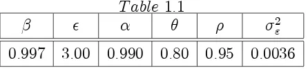
The frequency chosen to perform this exercise is monthly. The baseline calibration is shown in Table 1.1. Before discussing this calibration, it is worth mentioning that four out of six of the structural parameters are calibrated by using information from the Dominick´s database and some relationships derived from the model.9 These parameters are ; ; and 2". The main advantage of calibrating the majority of
8When …rms face idiosyncratic productivity shocks, a zero in‡ation policy cannot attain the natural
level of output. In fact, the second order approximation of the standard New Keynesian Phillips curve is di¤erent from the one derived when …rms are hit by idiosyncratic shocks. In the latter, there is a constant term than depends on the variance of the idiosyncratic shocks. Therefore, zero in‡ation cannot lead to a zero output gap, up to a second or higher order approximation. However, the impact of non zero output gap on the welfare function is of third or higher order with price stability.
9The Dominick´s database contains nine years (from 1989 to 1997) of weekly store level data on
parameters by using the same database is that it provides consistency between the di¤erent choices of parameters.
T able 1:1
2
"
0:997 3:00 0:990 0:80 0:95 0:0036
It is assumed that = 0:997, implying a steady state real return of …nancial assets of about four percent in annual terms. I set = 3, based on the evidence provided by Chevalier, Kayshap and Rossi (2003). They estimate price elasticities using the quantity and price data from Dominick´s database. Most of their elasticity estimates range between 2 and 4. I set so that it equals the average labor income share (0.66 in this calibration) times the markup implied by the choice of .10 On price stickiness, it is assumed = 0:8 such that the model matches the average price duration of …ve months estimated by Midrigan (2006) using the Dominick´s database.11 This price duration is also close to those found in the studies performed by Bils and Klenow (2004) and Altig et al.(2004). The persistence of the idiosyncratic component of productivity is assumed to be very high by setting = 0:95. This is the preferred point estimate of in Blundell and Bond (2000).12 They estimate an AR(1) process for the …rm´s idiosyncratic productivity by using a panel data covering 509 U. S. manufacturing companies observed for 8 years. Finally, the calibration of 2
" is performed such that
I match the observed variance of individual price changes. This is done by using the following expression derived from the model presented above:13
2
" =
(1 )(1 2)
2(1 )(1 ) 2 V arif (i)g 2 1
2
(1.39)
where V arif (i)g is the variance of monthly individual price changes across goods
and is the monthly in‡ation. Now, it is straightforward how 2
" is computed. Given
10Firms’pro…ts maximization in the steady state implies that1 =
1mctwhere mct denotes the
real marginal cost. Moreover, the assumption about technology implies that the real marginal cost is equal to the labor share (ls) divided by :Therefore, = 1ls.
11The average price duration is computed by considering regular prices only (no sales). See Midrigan
(2006) for the details on this calculation.
12They provide an estimate of equal to 0.565 in annual frequency. In order to translate this
estimate into the monthly frequency, I use a = 12m. This approximation assumes that productivity is end of period sampled and interprets it as a stock variable. I use"a" to denote annual frequency and"m"to denote monthly frequency.
[image:26.595.200.423.170.220.2]equation (1.39), the values set above for ; ; ; and ; a constant monthly in‡ation of 0.03/12 and a variance of monthly individual price changes across goods equal to 0.002116 (consistent with the observed standard deviation of monthly individual price changes of 4.6 percent found in the Dominick´s database), it yields 2
" = 0:0036. The
latter value is slightly lower than the one set by Golosov and Lucas (2007).14 Under this calibration, the welfare losses of price rigidities are equivalent to 1.7 percent of steady state consumption.
1.4.3.1 Robustness Exercise
Four important sources of uncertainty can a¤ect the baseline estimate. First, even assuming that the Dominick´s database is a representative sample of the economy, there exists uncertainty about the persistence of the idiosyncratic component of pro-ductivity and the elasticity of substitution.15 Second, there is uncertainty about the determinants of the observed heterogeneity in the size of individual price changes. In the baseline calibration, it has been assumed that the variance of the idiosyncratic productivity shock can account for almost all the variance of individual price changes. However, it is possible that there exist ex-ante heterogeneity, like di¤erent frequencies of price adjustment, that can help to explain this variance. Third, the estimates of and , obtained by using the Dominick´s database, are signi…cantly lower than oth-ers presented in alternative studies. Therefore, there is uncertainty about how well the economy is represented by the information contained in the Dominick´s database. Moreover, given the way I calibrate the variance of the …rm speci…c productivity shock, this third source of uncertainty introduces a fourth one on 2
" and its relation with
and . In this subsection, I analyze and discuss how the baseline estimate changes when we consider all these sources of uncertainty separately.
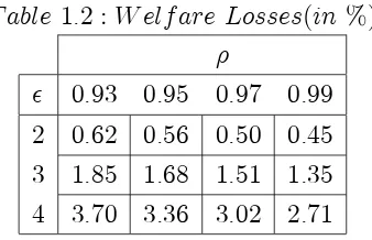
In order to show how much the …rst source of uncertainty may matter, Table 1.2 presents the welfare losses by allowing the parameters and to vary between
14They choose a variance equal to 0.011 in their baseline calibration in quarterly frequency. Then,
in order to translate my estimate into quarterly frequency and compare it with the one of Golosov and Lucas (2007), I apply the following relation: 2
"q = (1 + 2m+ 4m) 2"m. My monthly estimate is equivalent to a quarterly estimate of 0.010. I use "q" to denote quarterly frequency and "m"to denote monthly frequency.
15Notice that the uncertainty in and leads to uncertainty in 2
". Given that the latter is pinned down from all the other parameters and from the standard deviation of price changes, it is not considered that 2
reasonable values.16 In all these cases, and 2
" are also changed appropriately such
that the procedure followed to obtain the baseline estimate is the same, except in the choice of and . From this table, it can be seen that the welfare losses are very sensitive to the elasticity of substitution. This sensitivity is not signi…cantly a¤ected by the values of . The degree of autocorrelation of the …rm´s productivity is less important in order to determine the welfare losses for low values of .
T able 1:2 :W elf are Losses(in %)
0:93 0:95 0:97 0:99 2 0:62 0:56 0:50 0:45 3 1:85 1:68 1:51 1:35 4 3:70 3:36 3:02 2:71
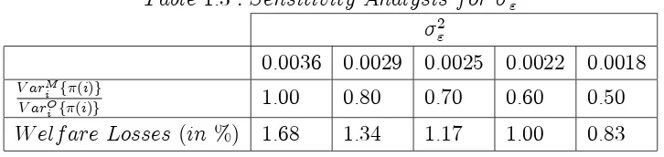
The second source of uncertainty is explored by analyzing how the baseline esti-mate changes when only the variance of the idiosyncratic productivity shock varies. Table 1.3 presents this sensitivity analysis. I consider …ve di¤erent values for 2" in
the table. The …rst column corresponds to the baseline estimate. The second row in the table indicates the fraction of the observed variance of individual price changes that is explained by the model. Clearly, in the baseline calibration, this fraction is 1, which means that basically all the observed heterogeneity is due to idiosyncratic shocks. However, it could be argued that there exists some ex-ante heterogeneity that can also account for the variance of the individual price changes. Midrigan (2006) performs an analysis by using the Dominick´s database and concludes that only 20 percent of the variance of price changes could be explained by ex-ante heterogeneity. This case corresponds to the calibration in the second column. Given that ex-ante heterogeneity is not incorporated in the model, I calibrate the variance of the idiosyn-cratic productivity shock such that only 80 percent of the variance of individual price changes is explained by the model. It can be seen that the estimate of the welfare losses diminishes to 1.34 percent of steady state consumption in this case. This result is not so di¤erent from the one obtained with the baseline calibration.
16The two standard error con…dence interval for , implied by Blundell and Bond´s estimation,
[image:28.595.227.396.247.356.2]T able 1:3 :Sensitivity Analysis f or 2
"
2
"
0:0036 0:0029 0:0025 0:0022 0:0018
V arM i f (i)g
V arO i f (i)g
1:00 0:80 0:70 0:60 0:50
W elf are Losses (in %) 1:68 1:34 1:17 1:00 0:83
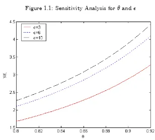
The third source of uncertainty is related with the convenience of employing the Dominick´s database to calibrate some parameters. There exist some evidence that can cast doubt on the usefulness of this database. In particular, this evidence suggests that the degree of price rigidity and the elasticity of substitution among goods are much higher than the ones estimated with the Dominick´s database. Nakamura and Steinsson (2007) report that the average price duration is between 11.6 and 13 months; while Klenow and Kristow (2007) …nd that the average price duration is 8.6 months. Golosov and Lucas (2007) mention that typically falls in the range between 6 and 10. This implies di¤erent values from for as well.17 Therefore, given the con‡icting evidence for and , it is necessary to perform a sensitivity analysis to the baseline calibration by changing only these parameters and accordingly. Notice that 2
"
,in this analysis, corresponds to the one used in the baseline estimate, given that the information on the variance of individual price changes is not available in the alternative studies. I evaluate later how welfare losses change when 2
" varies for
di¤erent values of and .
Figure 1.1 shows the results of this exercise. On the vertical axis, the welfare losses are measured as percentage of steady state consumption. The parameter is allowed to vary between 0.8 and 0.92, which implies that average price duration is between 5 and 13 months. The lines in the graph describe how welfare losses change with the degree of price rigidity for three di¤erent levels of the elasticity of substitution among goods. Two interesting results arise from this picture. First, for any degree of price rigidity, the estimation of the welfare losses is very sensitive to variations in in the range between 3 and 6; while it is not severely a¤ected when moves between 6 and 10. Second, the whole picture reveals that the uncertainty in and is translated in a huge uncertainty about the welfare losses, which vary from 1.7 percent( = 0:8; = 3) to 4.4 percent of steady state consumption ( = 0:92; = 10).
To conclude the robustness exercises, I quantify how movements in 2" a¤ect the
[image:29.595.108.471.131.217.2]Figure 1.1: Sensitivity Analysis for and
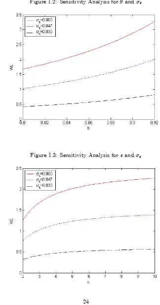
estimates of welfare losses for di¤erent degrees of and . Figures 1.2 and 1.3 present the results of these exercises. Figure 1.2 shows how welfare losses change with the degree of price rigidity for three di¤erent levels of ". It can be seen that the degree of price rigidity does not signi…cantly a¤ect the losses for low levels of volatility of the shock ( " = 0:03 or less). The picture considers = 3, but this result also holds if = 10. Moreover, the uncertainty in and " also implies an enormous uncertainty about the welfare losses, which vary from 0.4 percent to 3.3 percent of steady state consumption. Figure 1.3 presents how the losses vary with the elasticity of substitution for the same levels of ". This picture shows that the uncertainty in the elasticity of substitution does not matter much for low levels of ". Besides, the impact of the
Figure 1.2: Sensitivity Analysis for and "
[image:31.595.115.439.137.753.2]1.5
Welfare Losses with State-Dependent Pricing
In the previous section, the Calvo price-setting was used in order to estimate the welfare losses resulting from price stickiness. One weakness of this approach is that it does not incorporate the fact that it is more likely that those …rms that have their prices further away from their target prices have a higher probability of changing their prices.18 In this section, I use a modi…ed version of the Generalized Ss model proposed by Caballero and Engel (2007) in order to let the probability of changing prices be an increasing function of the di¤erence between the actual price and the target price. The section is divided into three parts. First, I present the model. Then, I show how to use it in order to compute the welfare losses. Finally, I present the baseline calibration of the model and some robustness exercises.
1.5.1
The Model
Consider a …rmi2[0;1]at timetthat sets its price atPt(i)but would choose its price
atPt(i)if price rigidities were momentarily removed. Let the di¤erence between these two prices (the actual and the target prices respectively) be de…ned, in logarithms, as follows:
xt(i) = pt(i) pt(i) (1.40)
For simplicity, in this section I assume that there exists idiosyncratic productivity shocks only, which are independent across …rms and across time. All these shocks have zero mean and variance 2". Moreover, under the assumption that increments in
productivity are approximately independent (over time for eachi), I can approximate
pt(i) by the following expression:19
pt(i)' +pft(i) (1.41)
where pft(i) is the log of the frictionless price (the price that a …rm would choose if price rigidities were permanently removed) and is an uninteresting constant. In
18The cost of deviating from the target price is increasing with respect to the distance from this
price. Therefore, adjustment is more likely when this distance is larger.
19This assumption has been used in other applications by Caballero and Engel (1993a,1993b). It
general, the target price would be a weighted average of current and expected future frictionless prices. When productivity is very persistent (in the limit it is a unit root), it can be shown that the expectation of the future frictionless prices is approximately the current price.20 Therefore, it holds that the target price is approximately given by the frictionless price.21
From (1.41), it holds that:
pt(i)' pft(i) (1.42) Notice from Section 2 that the frictionless price is given by:
pft(i) = log +wt+
1
( pt+ct)
1
at(i) (1.43)
Considering that there are no aggregate shocks and that in‡ation is equal to zero, it can be concluded that wt =w, pt = p and ct = c. The latter implies that the target
price follows the process:
pt(i)' pft(i) = at(i) (1.44)
Given that is very close to 1, at(i)'"t(i). Therefore:
pt(i)' "t(i) (1.45)
The existence of idiosyncratic productivity shocks every period implies that the target price changes every period; and, consequently the price imbalance x also varies. To complete the model, I need to specify how …rms would adjust their prices after being hit by the idiosyncratic shock. I assume that the probability that a …rmi changes its price is equal to (xt(i)) where (x) represents the adjustment hazard. In this way, I
capture the most distinguishing feature of state-dependent models: the fact that the disequilibrium variablext(i)in‡uences how likely it is that a …rm adjusts its price in a
given time period.22 In principle, a hazard function could take any shape. Reasonable hazard functions should be increasing with respect to the absolute value of x, given 20Notice that, in the limiting case, when the productivity is a unit root, the frictionless price is a
unit root.
21See Caballero and Engel (1993b) for more details on this issue.
22The adjustment hazard framework has been used by Caballero and Engel (1993a, 1993b, 2006,
that it seems unlikely that …rms tolerate large deviations as much as they tolerate the small ones.23 This feature is known in the literature as the increasing hazard property (Caballero and Engel 1993a).
The timing convention of the model is as follows. At the beginning of period t, …rm i has a price imbalance of xt 1(i). Then, an idiosyncratic productivity shock
hits the …rm. This implies that x moves from xt 1(i) to xt 1(i) + pt(i). Finally,
the adjustment hazard is applied on the price deviation after the idiosyncratic shock. With probability (xt 1(i)+ pt(i))the …rm changes its price and eliminates the price
imbalance24 ( x
t(i) = 0) and with probability 1 (xt 1(i) + pt(i)) the …rm does
not change its price and keeps its price deviation in xt 1(i) + pt(i). Therefore, for
each …rmi; the following process forxt(i) holds:
xt(i) =It(i) xt 1(i) "t(i) (1.46)
where:
It(i) = 1 with Probability 1 (xt 1(i) + pt(i))
= 0 with Probability (xt 1(i) + pt(i))
1.5.2
Measuring Welfare Losses
In this case, it is convenient to combine (1.17) with (1.18) in order to write the welfare losses as:
Lt=
2 V ari
n
pt(i) pft(i)
o + 1 +
2 (ybt yb
n t)
2 (1.47)
Again, these losses have two parts: one that depends on policy and one that does not. Equation (1.45) is consistent with zero in‡ation, which is assumed. Moreover, I assume that the standard New Keynesian Phillips curve is still a good approximation to relate output gap and in‡ation.25 Under this assumption, a zero in‡ation policy leads to a
23In fact, menu costs models are consistent with increasing hazard functions.
24When the price imbalance is positive (negative), eliminating this imbalance implies that the …rm
has decreased (increased) its price.
25Gertler and Leahy (2006) show that the standard New Keynesian Phillips curve is consistent
zero output gap, up to a …rst order approximation. Consequently, the welfare losses are given by:
Lt=
2 V ari
n
pt(i) pft(i)
o
(1.48)
This implies that the only source of welfare losses is the dispersion of price gaps across goods. Given that the model is de…ned in terms of the price deviation from the desired price (or target price), it is convenient to rewrite the welfare losses as a function of the cross sectional variance ofxt. By using (1.41) in (1.48), the welfare losses can be
expressed as:
Lt=
2 V arifxt(i)g (1.49)
1.5.3
Quantifying
V ar
if
x
t(i)
g
The cross sectional variance is estimated by …nding the variance of the ergodic distri-bution of the state variable x for a given …rm i. In order to simulate the process x I need to assume a functional form for (x): Following Caballero and Engel (2006), I assume the simplest quadratic hazard they present in their paper, which is given by the following expression:
(x) = px2 , x 0 (1.50)
= nx2 , x 0
The parameters and are the same as those in the baseline calibration in Section 4. The remaining parameters p; n and 2" are calibrated in two slightly di¤erent ways.
In the …rst one, I impose p = n and calibrate the parameters such that I match the
fraction of price adjustments and the standard deviation of individual price changes observed in the Dominick’s database.26 In the second one, I remove the restriction
p = n, such that I can match additionally the fraction of positive price changes.27
higher.
26Notice that the fraction of price adjustments (f) is approximately related to the average price
duration (d) by the following expression: f d 1
27Of course, there exists other dimensions of the data that could be matched. It would be interesting
T able 1:4 :Calibration of the Hazard M odels
Data Models
1 2 3
STATISTICS (In %)
Fraction of Price Adjustments 20 20 20 20 Standard Deviation of Price Changes 4.6 4.6 4.6 4.6 Fraction of Positive Price Changes 13 10 13 10
jMean of Price Adjustmentsj 7.7 9.8 9.0 7.6
Mean of Price Increase 9.8 6.8 7.6
Mean of Price Decrease 9.8 13.4 7.6
PARAMETERS
p 50 205
-n 50 15
-" 0.047 0.047 0.047
WELFARE LOSSES (In %) 0.28 0.37 1.33
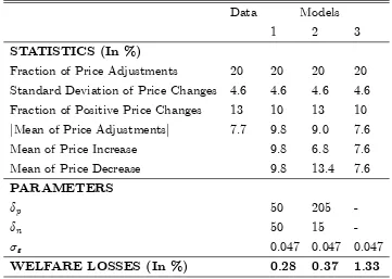
Table 1.4 summarizes the results of the simulations. Model 1 reports the symmetric quadratic hazard model. The model fails to match the mean of the absolute value of individual price changes (it overestimates it). This is consistent with the failure of menu costs models to generate many small price changes.28 By using this model, the welfare losses are 0.3 percent of steady state consumption. Model 2 reports the asymmetric quadratic hazard model. Notice that p is much higher than n in order
to capture the fact that price increases occur more frequently than price reductions. Moreover, the asymmetric hazard allows for matching the fraction of price increases, which is higher than the one of price decreases. Like Model 1, it predicts an absolute value of price changes that is much higher than the one observed in the data. With this model, the welfare losses are 0.4 percent of steady state consumption. Model 3 reports the constant-hazard model (Calvo 1983). This model has been calibrated so that (x) = 1 = 0:2. In contrast to the previous two models, it matches fairly well the mean of the absolute value of price adjustments. However, it does not capture (by construction) the higher probability of a price increase. By using this model, the welfare losses are much higher (1.3 percent of steady state consumption ). Finally, notice that the welfare losses estimated by using model 3 are a very good
[image:36.595.129.490.137.394.2]approximation to the ones estimated by using the complete structure of the Calvo model under the assumption that the idiosyncratic productivity is highly persistent. In fact, when using the adjustment hazard approach, the estimated losses are 1.33 percent; whereas when using the model of section 4 with = 0:99, these losses are 1.35 percent.
1.5.3.1 Robustness Exercise
In the previous calibration exercises, there exist two important sources of uncertainty. Conditional on the representativity of the Dominick´s database, the …rst source is the estimation of the elasticity of substitution. In fact, estimates of this parameter based on the use of the Dominick´s database are in the range 2-4. This implies, after following the same type of procedure performed in table 3, that the welfare losses are between 0.1 and 0.6 percent of the steady state consumption if model 1, with p = n,
is used. When model 2 is considered to perform this robustness analysis, the range for the welfare losses is 0.1-0.7 percent of the steady state consumption.
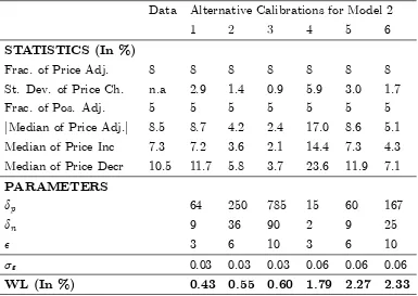
The second source of uncertainty is related with the convenience of using the Do-minick´s database. As mentioned before, other studies present estimates of the elastic-ity of substitution among goods and the average price duration that are much higher than those obtained by using this database. For this reason, I also perform some additional calibration exercises of the welfare losses that consider: a) lower frequency of price adjustments (average price duration equal to 13 months instead of 5 months) b) three di¤erent estimates for the elasticity of substitution among goods and c) two di¤erent values for ". All these exercises are performed by calibrating model 2 (with p 6= n) such that the fraction of price adjustments and the fraction of positive price
changes are the same as in the data on individual price changes due to Nakamura and Steinsson (2007). Results are presented in Table 1.5.
Several interesting results emerge from this robustness exercise. First, the impact of the degree of price rigidity on the welfare losses is crucially a¤ected by the size of the standard deviation of the idiosyncratic productivity shock. When " = 0:03;
of the welfare losses. In particular, calibrations 1 and 5 do a great job in matching the absolute value of the median of price adjustments and the median of price increases but yield completely di¤erent welfare losses (0.4 versus 2.3 percent). Independent evidence on the variance of the idiosyncratic productivity shocks is necessary in order to obtain a more precise estimate of the welfare losses. Third, given ", the impact of
varying on welfare is not very important. This result holds because in order to match the fraction of price changes and the fraction of positive adjustments, an increase in implies a reduction in the variance of the price imbalance xt. Fourth, this exercise
shows clearly that a lower frequency of price adjustments would not necessarily imply signi…cantly more welfare losses. If we compare the result obtained by using calibration 1 with the baseline estimate of 0.37 percent, we see that the di¤erence between the two is small. This is because it is plausible that economies with lower frequency of price adjustments are economies with smaller idiosyncratic productivity shocks. Fifth, the model does not …t the disaggregated data on prices when = 10. A higher variance of the idiosyncratic productivity shock will solve this problem. In general, when choosing any value for the elasticity of demand higher than 6, the model would require a higher
" in order to match adequately the data on individual price changes.
T able 1:5 :Robustness Exercise
Data Alternative Calibrations for Model 2
1 2 3 4 5 6
STATISTICS (In %)
Frac. of Price Adj. 8 8 8 8 8 8 8
St. Dev. of Price Ch. n.a 2.9 1.4 0.9 5.9 3.0 1.7
Frac. of Pos. Adj. 5 5 5 5 5 5 5
jMedian of Price Adj.j 8.5 8.7 4.2 2.4 17.0 8.6 5.1 Median of Price Inc 7.3 7.2 3.6 2.1 14.4 7.3 4.3 Median of Price Decr 10.5 11.7 5.8 3.7 23.6 11.9 7.1
PARAMETERS
p 64 250 785 15 60 167
n 9 36 90 2 9 25
3 6 10 3 6 10
" 0.03 0.03 0.03 0.06 0.06 0.06
[image:38.595.119.504.448.721.2]1.6
Concluding Remarks
I have presented a new perspective on the importance of the study of price rigidities. Traditionally, these rigidities have been analyzed in order to understand the real e¤ects of monetary policy, in‡ation persistence or the design of optimal monetary policy. In this sense, price stickiness has been an important element in monetary policy analysis. Here I provide an additional motivation to pay attention to price rigidities. In particu-lar, I emphasize that price stickiness is relevant because it can cause important welfare losses, even in economies with price stability. This conclusion has been obtained after considering idiosyncratic productivity shocks in the welfare analysis of price rigidities. The results of this paper also allow for the identi…cation of two aspects of price rigidities that are relevant from a welfare point of view. First, they highlight how crucial it is to understand why …rms would decide in favor of state dependent behavior or time dependent behavior.29 In fact, this study has shown that the welfare losses are signi…cantly higher with time dependent pricing. Secondly, they emphasize the importance of investigating the determinants of the frequency of price adjustments. According to my results, this variable is a key factor in determining the size of welfare losses.30 Research on these two aspects would also be helpful in order to see if there exist policies that can help to reduce the negative impact of price rigidities.
29Alvarez (2007) develops an econometric analysis in this line of research. He estimates a
multino-mial logit model with Spanish Survey data in order to explain the relationship between the use of time dependent pricing strategies and industry characteristics. He …nds that time dependent behavior is associated with higher labor intensity in the production, lower degree of competition and large …rms.
30The other factor is the variance of the idiosyncratic productivity shocks. Clearly, this factor is
Chapter 2
Testing for Rule of Thumb
Price-Setting
2.1
Introduction
Much of the recent literature on monetary policy uses the New Keynesian Phillips curve (NKPC) to describe the aggregate supply block of the economy. Many authors, however, have criticized the NKPC on the basis that it cannot explain the degree of inertia observed in in‡ation. In particular, Fuhrer and Moore (1995) show that the NKPC predicts a degree of persistence in in‡ation that is much lower than the one detected in the data. To overcome this empirical de…ciency, three alternative strate-gies have been developed. First, the work of Galí and Gertler (1999) incorporates backward-looking behavior by assuming that a fraction of …rms follows a simple rule of thumb. Alternatively, Smets and Wouters (2003) and Christiano et. al. (2005) as-sume that …rms partially index prices to past in‡ation when not re-optimizing. Either through rule of thumb behavior or indexation, the modi…ed in‡ation equation, known as the hybrid NKPC, can rationalize a lagged in‡ation term and account for persis-tence in in‡ation. The third strategy is the one followed by Mankiw and Reis (2002). They build the sticky information model in which …rms are assumed to update their information sets infrequently, due to the presence of costs of collecting and processing information.
macroeconomic data.1 The main conclusion is that all these models are useful in order to replicate in‡ation dynamics with plausible parameters. However, how good are these strategies in matching the microeconomic evidence on price-setting? According to Alvarez (2007), all these models fail to match some of this evidence. Models with indexation as well as sticky information models fail in matching infrequent adjustment, a decreasing hazard rate, annual spikes in hazard rate, and heterogeneity in price adjustment.2 Instead, the model of Galí and Gertler (1999) only fails in capturing a decreasing hazard rate and annual spikes in hazard rate. Therefore, the latter model seems to be much in accord with the microeconomic evidence.
In this chapter, I propose a novel methodology in order to evaluate the quantitative importance of the rule of thumb behavior proposed by Galí and Gertler (1999).3 By using their hybrid model, I derive a structural relationship over time between the cross sectional variance of individual price changes and aggregate in‡ation. There are four important features of this relation that make it more attractive than the hybrid NKPC in order to identify rule of thumb behavior. First, the parameters that appear in the equation I derive are only those related with the nature of price-setting: the one that measures the degree of price stickiness and the one that measures the fraction of backward-looking …rms. Both of them are identi…ed directly from estimates of that equation. The latter means that the estimates of these parameters are not a¤ected by how real rigidities are modeled and calibrated, as it is the case when they are identi…ed by estimating the hybrid NKPC.4 Second, the variables that appear in the relationship I propose are predetermined in periodt. This implies that I do not need an assumption on how expectations about the future are formed. Instead, the estimation of the hybrid NKPC requires to take a position on this issue, given that expected in‡ation appears in that relation.5 Third, estimating the equation I propose is not
1See Galí and Gertler (1999), Galí et al. (2001), Smets and Wouters (2003), Christiano et. al.
(2005), and Mankiw and Reis (2002).
2The sticky information model additionally fails in not allowing the presence of non optimal price
setters.
3Evaluating the plausability of rule of thumb …rms is not only useful to study in‡ation persistence
but also for monetary policy analysis. Steinsson (2003) shows that optimal monetary policy change in important ways if some …rms obey a rule of thumb.
4See Galí and Gertler (2001), Galí and Lopez Salido (2001), and Benigno and Lopez Salido (2006). 5Galí and Gertler (1999), Galí et al. (2001), Galí and Lopez Salido (2001), Galí et al. (2005), and
subject to the criticism of Rudd and Whelan (2005), who claim that …tting the hybrid NKPC may be biased in favor of …nding a signi…cant role for forward-looking behavior. Fourth, the de…nition of the variables I use do not change for alternative assumptions on the degree of openness, the form of the production function and the way how real rigidities are introduced. Instead, the construction of measures of real marginal costs in the hybrid NKPC is very sensitive to the previous assumptions.6
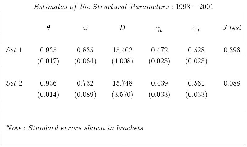
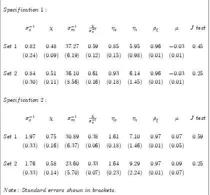
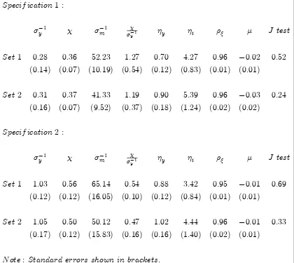
I estimate the derived structural relationship with Spanish monthly data covering the period 1993-2001. The estimation technique is the Generalized Method of Mo-ments (GMM). Several interesting results stand out. First, the structural relationship proposed in this paper …ts the data well. Second, the backward-looking price set-ting is statistically signi…cant and quantitatively important. Third, the estimates of the fraction of rule of thumb …rms are very close to those found by Galí and Lopez Salido (2001) and Benigno and Lopez Salido (2006) by estimating the Spanish hybrid NKPC. Fourth, the degree of price stickiness implied by the estimates is consistent with the average price duration estimated using only disaggregated data. Fifth, the estimates imply that forward-looking behavior is only slightly dominant in shaping in‡ation dynamics in Spain.
The rest of the chapter is organized as follows. In Section 2.2, I present the model and the basic assumptions. In Section 2.3, I derive analytically the dynamic relation-ship between the cross sectional variance of individual price changes and aggregate in‡ation. In Section 2.4, I expose the methodology and the econometric speci…cation used in order to estimate the degree of backward-lookingness. The estimates and re-lated comments are also presented in this section. In Section 2.5, I present a detailed comparison of the methodology that I propose and the one developed by Galí and Gertler (1999), who estimate the hybrid NKPC. Conclusions are given in Section 2.6.
2.2
The New Keynesian Hybrid Model
In this section I brie‡y describe the hybrid model developed by Galí and Gertler (1999). This model is used in the next section in order to derive the dynamic structural
rela-reduced form of the hybrid NKPC.
6Galí and Lopez Salido (2001) show that the de…nition of real marginal cost can change with
tionship between the cross sectional variance of individual price changes and aggregate in‡ation.
2.2.1
Households
The household purchases di¤erentiated goods and combines them into composite goods using a Dixit-Stiglitz aggregator:
Ct =
0 @
1
Z
0
Ct(i)( 1)= di
1 A
=( 1)
(2.1)
where Ct(i) is the di¤erentiated good of type i and >1 is the constant elasticity of
substitution among goods. The households maximize the index (2.1) given the total cost of all di¤erentiated goods and their nominal prices Pt(i). Then, the demand for
each good is given by:
Ct(i) =
Pt(i)
Pt
Ct (2.2)
where Pt is the aggregate price level and is de…ned as follows:
Pt=
0 @
1
Z
0
Pt(i)1 di
1 A
1=(1 )
(2.3)
2.2.2
Firms
In the model, it is assumed a continuum of …rms indexed by i 2 [0;1]: Each …rm is a monopolistic competitor and produces a di¤erentiated good Yt(i) that sells at price
Pt(i). Firms set prices as in the sticky price model of Calvo (1983). In this model,