Essays on Familiarity and Choice

Texto completo

(1)Essays on Familiarity and Choice. Francesco Cerigioni. ADVERTIMENT. Lʼaccés als continguts dʼaquesta tesi queda condicionat a lʼacceptació de les condicions dʼús establertes per la següent llicència Creative Commons: http://cat.creativecommons.org/?page_id=184 ADVERTENCIA. El acceso a los contenidos de esta tesis queda condicionado a la aceptación de las condiciones de uso establecidas por la siguiente licencia Creative Commons: http://es.creativecommons.org/blog/licencias/ WARNING. The access to the contents of this doctoral thesis it is limited to the acceptance of the use conditions set by the following Creative Commons license: https://creativecommons.org/licenses/?lang=en.

(2) U NIVERSITAT A UTÒNOMA DE B ARCELONA D OCTORAL T HESIS. Essays on Familiarity and Choice. Author: Francesco Cerigioni. Advisor: Prof. Miguel A. Ballester. Tutor: Prof. Omar Licandro. A thesis submitted in fulfillment of the requirements for the degree of Doctor of Philosophy in the International Doctorate in Economic Analysis Departament d Econòmia i Historia Econòmica. 2016.

(3) ii. On the importance of theory: “There are no facts, only interpretations.” Friedrich W. Nietzsche On the inevitability of habits: “Habits gradually change the face of one’s life as time changes one’s physical face; one does not know it.” Virgina Wolf On the shortcomings of this thesis: “Every man is guilty of all the good he didn’t do.” Voltaire.

(4) iii. Acknowledgements I am grateful to the Universitat Autònoma de Barcelona for the grant for Trainee Reserach Staff given to me during the Academic Year 2010-2011 and to the Ministerio de Ciencia y Innovación for the FPI scholarship BES2011048581 given to me during the Academic Years 2011-2015. Both financial aids allowed me to pursue the research presented in this thesis. I will be forever in dept with my advisor and, more importantly, friend Miguel A. Ballester that has been a guide and mentor. Thank you Miguel A. for never throwing me out of your office, not even when I gave up working and just started complaining about everything. Thank you for never giving up on me and my, sometimes crazy, ideas and for always being able to push me and direct me in the right direction. Thank you for teaching me how to talk with the profession. Thank you for giving me focus. Thank you for having been much much more than an advisor. IDEA and UAB will miss you. I want also to thank Kfir Eliaz, Itzhak Gilboa and Ariel Rubinstein for the incredible amount of effort they put in guiding me and helping me improving my main work. It has been not only a great pleasure to have this opportunity but also an incredible honor. Thank you Kf1r for having probably spent countless hours in reading the papers, their weaknesses and how to present the ideas inside them. Thank you for your suggestions, patience and for helping me in every possible way to prepare for the market. Moreover, thank you for your friendship and kindness. Nevertheless, I cannot thank you (neither my family) for having awakened my addiction to Formula 1 that I thought I had been able to control. The discovery of my incapability of controlling my addiction has destroyed the self image I had even if it probably improved some of the insights of the thesis. Thank you Tzachi for always having tried to understand the incomprehensible and messy research notes I was presenting you during my visit in Tel Aviv. Your comments were always great and helped me improve the papers considerably. Thank you so much for all the interesting conversations we had during our coffees regarding philosophy, Italian history and humanism. They opened up my mind and filled it with countless stimuli. Thank you Ariel for our coffees together, your ideas and critiques and all the insights you gave me that greatly improved this thesis. Thank you for presenting me many researchers that helped me a lot during my Ph.D. Moreover, thank you for all the conversations we had on Israeli history and in particular for all the tips you gave me for my Jerusalem visit. They made it unforgettable. Furthermore, I want to thank Caterina Calsamiglia and Pedro Rey for having been my mother and father during this long process we call Ph.D. They not only helped me developing the ideas in the papers and read all the horrible versions I wrote through the years, but also encouraged me not to give up and to pursue my dreams and hopes. Thank you Caterina for having been always open to discuss with me about anything. Thank you for helping me understanding the profession in a much deeper way than I would have ever dreamed of. Finally, thank you for always helping me with a smile..

(5) iv Thank you Pedro for all the advices you gave me and for all the time you spent with me discussing about ideas but also doubts. Thank you for guiding me and helping me understand my priorities and hopes. Thank you for being a friend. Thank you Àngels and thank you Mercè for everything. Thank you for being the soul of IDEA and for always trying to keep the pieces together. Without you this program would not exist. Thank you for letting your office be the place where help, bureaucratic but also psychological, could always be found. I will miss you, so I will bother you from time to time. Furthermore, I want to thank Angela for the incredible amount of help she gave me throughout the years. I want to thank all my friends that shared with me the experience of trying to become an adult in the world of research. Thank you Alberto, Alex, Benji, Dilan, Edgardo, Francesco, Isabel, Javi, John and Yuliya. Unfortunately, we just discovered that the growth process never stops. I would also like to thank all the people in IDEA and not that helped me in all these years of research where I felt part of a big family. Thank you Antonio, Daniel, Fabrizio, Guillem, Johannes, Jose, Larbi, Marco, Matthew, Tomás and Tugce. Moreover, I want to thank all the directors of the program that always helped me if possible. Last but not least I want to thank my incredible family. My wife Karina that is still with me, even after all the pressure this process meant for us. Thank you Kari for always being there with a smile and your hand open. Thank you for being so special that only being besides you makes me already a better person. Thank you for being the sun in the sky of my dark days. Thank you for being generous and for giving some of your light to our incredible daughter Sofia. Thank you Sofia for your laughs and kisses, hugs and innocence that have been fundamental in this last very stressing year. Thank you for showing me how to live. Thank you for teaching me how to be your father. Finally, I want to thank my parents, my sister and my nephew for having always been supportive and the best family I could have ever dreamed of. Thank you Mamma, Papà, Betta and Daki for being you..

(6) v. Contents Acknowledgements. iii. Introduction. vii. 1. 2. 3. Dual Decision Processes: Retrieving Preferences when some Choices are Intuitive 1.1 Introduction . . . . . . . . . . . . . . . . . . . . . . . . . . . . 1.2 Related Literature . . . . . . . . . . . . . . . . . . . . . . . . . 1.3 Dual Decision Processes . . . . . . . . . . . . . . . . . . . . . 1.4 The Revealed Preference Analysis of Dual Decisions . . . . . 1.5 A Characterization of Dual Decision Processes . . . . . . . . 1.5.1 On Conscious and Intuitive Behavior . . . . . . . . . 1.5.2 Estimation of the Similarity Function . . . . . . . . . 1.6 Extensions . . . . . . . . . . . . . . . . . . . . . . . . . . . . . 1.6.1 A Forgetful Decision Maker . . . . . . . . . . . . . . . 1.6.2 Revealing S1 and S2 with Partial Information on the Similarity . . . . . . . . . . . . . . . . . . . . . . . . . 1.7 Final Remarks . . . . . . . . . . . . . . . . . . . . . . . . . . .. 20 23. Dual Decision Processes and Noise Trading 2.1 Introduction . . . . . . . . . . . . . . . . . . . . . . . . . . 2.2 The Economy: OLG and Dual Processes . . . . . . . . . . 2.3 The Equilibrium . . . . . . . . . . . . . . . . . . . . . . . . 2.3.1 A Consistent Pricing Function . . . . . . . . . . . 2.4 Discussion: Underreaction and Overreaction . . . . . . . 2.4.1 Equity-Premium Puzzle and Analogical Thinking 2.5 Final Remarks . . . . . . . . . . . . . . . . . . . . . . . . .. . . . . . . .. 25 25 27 30 31 32 36 38. . . . . . . .. 39 39 41 42 43 47 48 50. Stochastic Choice and Familiarity: Inertia and The Mere Exposure Effect 3.1 Introduction . . . . . . . . . . . . . . . . . . 3.1.1 Related Literature . . . . . . . . . . . 3.2 Stochastic Choice and Exposure Effect . . . 3.3 Exposure Effect, Inertia and Heterogeneity 3.4 Characterization . . . . . . . . . . . . . . . . 3.4.1 Discussion: Menu Exposure . . . . . 3.5 Final Remarks . . . . . . . . . . . . . . . . .. . . . . . . .. . . . . . . .. . . . . . . .. . . . . . . .. . . . . . . .. . . . . . . .. . . . . . . .. . . . . . . .. . . . . . . .. . . . . . . .. 1 1 4 5 8 13 16 17 18 18. A Appendix to Chapter 1. 51. B Appendix to Chapter 2. 57. C Appendix to Chapter 3. 61. Bibliography. 65.

(7)

(8) vii. Introduction This thesis studies the channels through which familiar experiences influence individual behavior through automatic psychological processes with the aim of getting a clearer understanding of some puzzling economic phenomena. In particular, the research focuses on understanding two main channels that are discussed in the next two sections: (i) how familiar experiences influence individual behavior through similarity comparisons and, (ii) how familiar experiences influence individual behavior through the effect of exposure on the perceived value of the alternatives.. FAMILIARITY AND S IMILARITY Whenever we face decision problems that we perceive as similar enough with some others we have experienced, we tend to make intuitive decisions, that is, we tend to replicate past choices even if it is possible that new and better options are available. Thus, an important question arises. How does intuition affects individual behavior and, thus, market outcomes? In particular, two questions need to be addressed. What is the relationship between intuition and observed behavior? How does intuitive individual behavior affect aggregate market outcomes? Chapter 1 answers the first question. In doing so it addresses a closely related question that is still open in the literature (Bernheim and Rangel 2009, Rubinstein and Salant 2012, Masatlioglu, Nakajima, and Ozbay 2012 and Apesteguia, Ballester, et al. 2015) and that is extremely important for welfare analysis; how can we understand individual preferences from observed choices? If some decisions are intuitive and not driven by preferences the question is relevant and not trivial. If people make intuitive choices when they experience familiar decision problems, how can we understand their preferences? When we observe a decision maker sticking to past choices even when new alternatives are available, is it because he prefers what he chose in the past or is it because he chose intuitively thus disregarding new options he might prefer? To answer such questions it is important to study two issues: (i) how intuitive choices arise and (ii) how to distinguish conscious and intuitive choices from observed behavior. In chapter 1 we address the first issue by providing a new model of decision making that is a simple formalization of an important theory in cognitive sciences known as Dual Process Theory (Evans and Frankish 2009 and Kahneman 2011) that still, to the best of our knowledge, has no tractable formalization in economics. Following such theory, individuals are described by the interaction of two systems. System 1 is associative and unconscious. System 2 is analytic, conscious and demanding of cognitive capacity. The model proposed summarizes such theory. System 1 uses a similarity function and a similarity threshold that represents the cognitive costs of activating the other system, to assess whether new experiences are similar enough with those past ones which behavior can be replicated. If the similarity is high enough, System 2 is not activated and past behavior is replicated. On the other hand, if the similarity is not high enough, then System 2 drives the decision process rationally, by maximizing a preference relation. In this.

(9) viii formulation, intuitive choices arise because of System 1, thus, if we want to understand individual preferences and start to address the second issue, i.e. how to distinguish between conscious and intuitive choices, we need to understand which choices were made by System 2. We propose a way of analyzing choice data that is based on the analogies System 1 makes and thus, given similarity comparisons are made with past experiences, it uses the sequence in which choices have been made. The intuition of the method is as follows. Whenever we know that in some moment in time preferences were maximized, we know that the decision problem in question was not similar enough with its past. Thus, all those decision problems that are even less similar with their past should be the outcome of maximization of preferences too. Using this simple principle we can find a set of choices that are informative for the elicitation of individual preferences. Furthermore, the method is applicable to find a set of intuitive choices. In fact, in a similar fashion than before, whenever we know some choices were intuitive, all those decision problems that are even more similar with their past must have been solved intuitively by the decision maker. Such information is useful to understand from choice data what is considered similar enough by the agent which is an important piece of information whenever we want to predict individual behavior. In particular it allows us to get information regarding the cognitive costs the decision maker incurs when making thoughtful, non-intuitive choices. As an additional contribution, we provide an axiomatic characterization of the model that makes it falsifiable. In particular, we show that whenever the similarity function is known, a computationally simple weakening of the Strong Axiom of Revealed Preference is enough to characterize the entire model. The main intuition is that we should not observe inconsistent, i.e. cyclic, choices among the ones that have to be explained by maximization of preferences. Moreover, whenever social data are available, even if the similarity function is unknown, the model can be characterized by two simple consistency requirements that allow for the perfect identification of individual preferences and similarity comparisons. Finally, we show that the theoretical results are not heavily affected by assuming imperfect memory of the decision maker or partial knowledge of the similarity function. The simple model proposed in chapter 1 allows for the study of the implications of intuitive decisions for market outcomes, that is the second broad research question presented at the beginning of this section. Many different puzzling phenomena are observed in the markets that might be related to the kind of sticky behavior the model implies, but in chapter 2 we focus on the implications of intuitive decisions for financial markets. In particular, we study an economy similar to the one described in De Long et al. 1990 where overlapping generations of traders which behavior is the outcome of the interaction between System 1 and System 2, live two periods and have to decide how much of two assets to buy, one risky and one riskless, in order to maximize last period consumption. We show that even if traders receive perfect information regarding first and second period dividends generated by the risky asset, due to the similarity between different market environments, they can fail to update their beliefs and thus behave intuitively. Hence prices in equilibrium can be far from their fundamental value because some decisions are not taking all available information into.

(10) ix account. Moreover, prices depart from fundamentals in a predictable manner as some literature in the past years have suggested. In particular, we model traders whose System 1 makes similarity comparisons between market environments, thus whenever the change in the environment is not enough to be perceived, traders do not update their beliefs and behavior is driven by System 1. They trade on old information that is irrelevant for the new market environment. Otherwise, decisions are driven by System 2 and traders behave rationally. In this sense, the model proposes a channel through which noise trading emerges endogenously in contrast to the exogenous proportion of noise or inattentive traders usually assumed in the literature (for example De Long et al. 1990 and DellaVigna and Pollet 2009). The paper then shows that in equilibrium, when noise trading emerges due to similarity between different market environments, prices should follow some patterns that have been observed in the data. To be more specific, prices should be more volatile than in the perfectly rational framework (for example Shiller 1992), they should underreact in the short-run to new information (for example Cutler, Poterba, Summers, et al. 1991 and Bernard 1993) while they might overreact to new information in the long-run (seminal contribution by De Bondt and Thaler 1985). The intuition behind these results is as follows. First, prices are more volatile because there are two sources of risk in the economy. One is standard and is due to the dividend generating process. The other one is novel and is due to the endogenous formation of noise traders in the economy. Even if traders know how noise traders emerge, they cannot predict without uncertainty what will be their relative weight in the future and so prices vary more than in an economy where such uncertainty is not present. Second, prices underreact to news in the short-run because of the behavioral model that describes traders behavior. If new information arrives in the market not all traders will use it because for some of them the change of the market environment is not enough to be perceived. Thus, some traders will not use all the information and so prices would be stickier than a rational framework would imply. Third, overreaction in the long-run can occur because of the interaction of underreaction and new information arriving in the market. Due to underreaction, information is gradually incorporated into prices from one period to the next (momentum), thus when new information is available its effects on prices can sum up with old information being incorporated hence causing the movement in prices to be more pronounced than in a fully rational economy. Finally, we conclude the chapter with an analysis of the implications of these results for the equity-premium puzzle (Mehra and Prescott 1985). In particular, we discuss the fact that the equity-premium should be countercyclical in the economy described in the paper, something that is qualitatively in line with evidence presented in the last decades (Mehra and Prescott 2003).. FAMILIARITY AND I NERTIA Since Samuelson and Zeckhauser 1988 and Kahneman, Knetsch, and Thaler 1991 a lot of evidence has been found pointing to the fact that individual decision making exhibits a strong kind of behavioral inertia, i.e. the status-quo bias or the endowment effect, which source is not clear. Our.

(11) x choices are shaped by the experiences we had in a way that is more subtle that the mere acknowledgment of the fact that we learn through our experiences. Past choices become important for present ones because they become familiar and the effect of familiarity on choice is unconscious. In chapter 3, we propose a possible cognitive foundation for this particular kind of inertia that is called the mere exposure effect that has been discovered by Zajonc 1968 and that became a central process in cognitive sciences to understand the effects of familiarity on choices. The mere exposure effect can be described as the phenomenon by which people tend to develop a preference for things merely because they have been exposed to them, they are familiar with them. We use this idea to model a decision maker that chooses stochastically between alternatives and that the more he chose an alternative, i.e. the he has been exposed to it, the higher the probability of choosing it.1 The model we propose can be seen as a more general kind of status-quo bias, thus helping explain the endowment effect, loss aversion and present bias in a dynamic framework. We formally discuss these possibilities and then we show how such framework not only highlights the importance of experiences on choices through its dynamic dimension but it can also help to substantiate this idea by providing a precise theoretical prediction of what kind of heterogeneity should emerge from a population of otherwise identical individuals that had different experiences. This implication of the model is of particular interest for the literature that analyzes the impact of the first years of life on successive social and economic outcomes through individual decisions, e.g. Heckman 2006. In particular this result makes possible to understand and quantify the effect of experiences on the kind of behavioral inertia that is the focus of the chapter. Finally, we show how to falsify the model when we have data on choice probabilities of an homogeneous population that chooses from sequential choice problems. In particular, we propose four simple properties that fully characterize the model. The first of this properties is a generalization of the concept already introduced in Luce 1959 of independence of irrelevant alternatives (IIA) which states that the relative probability of choosing an alternative over another should not depend on the other alternatives in the set. The only change we impose is that the property has to be satisfied for any given level of exposure. The second property we propose is simply saying that exposure cannot decrease the probability of choosing an alternative. This is the key property capturing the exposure effect. The third property says that the effect of exposure should not be alternative specific. Finally, the fourth and more technical property, imposes that the effect of exposure cannot be marginally increasing. We then discuss the possibility of considering a more general kind of exposure, i.e. exposure to all the alternatives of the menu. To ease the reading of the chapters all proofs have been moved to the appendix while, for the same reason, figures and tables have been kept in the main text.. 1. In the chapter we also discuss a more general interpretation of exposure..

(12) 1. Chapter 1. Dual Decision Processes: Retrieving Preferences when some Choices are Intuitive 1.1. Introduction. Few of the choices we make every day are the result of a conscious decision making process. Automatic or intuitive decisions are ubiquitous. Think about daily routines, many times we just intuitively stick to decisions we have only consciously thought of once. This mechanism is true not only for marginal decisions. As highlighted by Simon 1987, managers take many intuitive decisions when deciding investment strategies for their firms. Moreover, according to Kahneman 2002, experts such as managers, doctors or policy makers often make intuitive decisions or follow their hunches due to their extensive experience. Thus, understanding automatic or intuitive decisions can be crucial to achieve a better understanding of individual behavior and in particular of market outcomes. Actual market equilibria might be far from the ones standard models predict if intuition plays a role in the decisions taken by the different economic agents. Hence, a question arises, what makes choices intuitive? The dichotomy between fast and intuitive decisions versus slow and conscious ones has been formally studied in cognitive sciences at least since Schneider and Shiffrin 1977. The seminal work by Evans 1977 and the successive models and findings in McAndrews, Glisky, and Schacter 1987, Evans 1989, Reber 1989, Epstein 1994 and Evans and Over 1996 stimulated the creation of a coherent theory of the individual mind as an interaction of two systems called Dual Process Theory that is described in Evans and Frankish 2009 and Kahneman 2011. System 1 is associative and unconscious. System 2 is analytic, conscious and demanding of cognitive capacity.1 Using analogies, System 1, source of intuitive choices, draws from past behavior to influence decisions. System 2, source of conscious choices, is costly and hence is only activated to solve problems for which past experience cannot be used by System 1. The associative nature of System 1 makes analogies extremely important for individual behavior and it highlights the centrality of the timing of decision problems to understand choices. 1. The names of the two systems appeared for the first time in Stanovich 1999. See Evans and Frankish 2009 to get a deeper description of the two different systems and of the historical development of the theory..

(13) 2. Chapter 1. Dual Decision Processes: Retrieving Preferences when some Choices are Intuitive. Past behavior can influence present choices because intuitive decisions are driven by the analogies System 1 makes. Thus, if we want to understand the role of intuitive decisions in markets, we need first (i) to have a model of intuitive choices that takes into account the role of past choices on present ones and (ii) to analyze whether it is possible from observed behavior to distinguish between conscious and intuitive choices. 2 These are the research questions we address in this chapter. To answer the first question we propose a simple formalization of Dual Process Theory. To the best of our knowledge there is no tractable formalization of such theory, thus the first contribution of the present chapter is to propose a formal model that can be used in standard economic analysis. In section 3.2, we model a decision maker composed by the two described systems. System 1 compares every decision environment with the ones that the decision maker has already faced according to some given similarity measure. Behavior is replicated from those past problems that are similar enough to the present one, i.e. the similarity between the problems passes some threshold that represents the cost of activating the other system. If there are no such problems, System 2 chooses the best available option by maximizing a rational preference relation. Think for example of a consumer that buys a bundle of products from a shelf in the supermarket. The first time he faces the shelf, he tries to find the bundle that best fits his preferences. Afterwards, if the price and arrangement of products do not change too much, he will perceive the two decision problems as if they are the same and so he will intuitively stick to the past chosen bundle. If on the contrary, the change in price and arrangement of the products is evident to him, he will choose by maximizing his preferences again. Even in such a simple framework, there is no trivial way to distinguish which choices are made intuitively and which ones are made consciously. Following the example, suppose our consumer faces again the same problem but this time a new bundle is available and he sticks with the old choice. Is it because the old bundle is preferred to the new one? Or is it because he is choosing intuitively? We show how to restore standard revealed preference analysis and thus answer the second research question by understanding in which decisions System 2 must have been active. Section 1.4 assumes that (i) the decision maker behaves according to our model and (ii) the similarity function is known while the threshold is not, i.e the cognitive costs of activating System 2 are unknown.3 We then show that, for every sequence of decision problems, it is possible to identify a set of conscious observations and the interval in which the cognitive costs should lie. To the best of our knowledge this is the first work attempting to assess such costs from observed behavior. We do this by means of an algorithm that uses the analogies made by System 1. First notice that new observations, i.e. those in which the choice is an alternative that had never been chosen before, must be generated by System 2. No past behavior could have been replicated. Starting from these observations, the algorithm iterates the following idea. If an observation is generated by System 2, any other more novel observation, that is any problem which is less similar to those decision problems 2 See Rubinstein 2007 and Rubinstein 2015 for a similar distinction between conscious and intuitive strategic choices for players participating in a game. See also the distinction in Cunningham and Quidt 2015 between implicit and explicit attitudes. 3 See sections 3.2 and 1.4 for a justification of the latter hypothesis..

(14) 1.1. Introduction. 3. that preceded it, must be also generated by System 2. Novelty depends on two factors: (i) how System 1 makes associations and (ii) the sequence of decision problems the decision maker has faced. These two are the factors the algorithm exploits to find conscious choices. Returning to our consumer, if we know that after a change in the price of the products on the shelf, the consumer chose consciously, then he must have done so also in all those periods where the change was even more evident. The algorithm identifies a set of intuitive decisions, i.e. those made by System 1, in a similar fashion, that is, first it highlights some observations that have to be intuitive and then uses this information to reveal other intuitive observations. In doing this, we consider cyclical datasets, i.e. datasets in which the standard revealed preference relation is cyclic. Notice that any cycle must contain at least one intuitive observation, given that observations generated by System 2 cannot create cycles in the revealed preference. Then, a least novel observation in a cycle, i.e. one that is more similar to its past among those forming a cycle, must be intuitive. Once we know that one observation is generated by System 1, so must be all observations not included in the cycle that are even less novel. Thus, the algorithm finds a set that contains only conscious observations and, in a dual way, another one that contains only intuitive ones. Interestingly enough, if the sequence meets some richness conditions, such sets contain all conscious and intuitive observations respectively. Obviously, knowing these two sets gives us crucial information regarding individual preferences and the degree of similarity that is needed to activate System 2. In fact, understanding if some decisions were made intuitively is very important to understand how analogies are made. Even if intuitive choices do not reveal individual preferences, they tell us what problems are considered similar enough by the decision maker. What is similar enough depends on the similarity threshold, thus intuitive choices provide crucial information regarding the unknown cognitive costs of activation of System 2. It is important to notice that the preference revelation strategy we use in the chapter agrees with the one used in Bernheim and Rangel 2009. They analyze the same problem of eliciting individual preferences from behavioral datasets, and they do this in two stages. In a first stage they take as given the welfare relevant domain, that is the set of observations from which individual preferences can be revealed, and then in a second stage they analyze the welfare relevant observations and propose a criterion for the revelation of preferences that does not assume any particular choice procedure to make welfare judgments.4 Even if similar, our approach differs in two important aspects. First, by modeling conscious and intuitive choices, we propose a particular method to find the welfare relevant domain, i.e. the algorithm highlighting a set of conscious choices. Second, by proposing a specific choice procedure, we use standard revealed preference analysis on the relevant domain, thus our method, by being behaviorally based, is less conservative for the elicitation of individual preferences. In this sense, our stance is also similar to the one proposed in Rubinstein and Salant 2012, Masatlioglu, Nakajima, and Ozbay 2012 and Manzini and Mariotti 2014 4 Notice that Apesteguia, Ballester, et al. 2015 propose an approach to measure the welfare of an individual from a given dataset that is also choice-procedure free. They do so by providing a model-free method to measure how close actual behavior is to the preference that best reflects the choices in the dataset..

(15) 4. Chapter 1. Dual Decision Processes: Retrieving Preferences when some Choices are Intuitive. that make the case for welfare analysis based on the understanding of the behavioral process that generated the data. Thus, falsifiability of the model becomes a central concern. In section 1.5 we propose a testable condition that is a weakening of the Strong Axiom of Revealed Preference that characterizes our model and thus renders it falsifiable. Moreover, we show that if the data are rich enough, in particular if we observe choices made by an homogeneous population, two simple consistency requirements not only characterize the model but also allow us to uniquely identify individual preferences and how analogies between decision problems are made. Section 1.5 concludes with a discussion on what conscious and intuitive behavior can be in a more general context that relies on our framework in section 1.5.1 and with the formal analysis of how to estimate the similarity function from an heterogeneous population of individuals sharing it in section 1.5.2. Section 1.6 discusses some possible extensions of the base model. First, we analyze the possibility of a decision maker with imperfect memory, that is, that recalls only the m most recent decision problems. We show that such extension does not hinder our algorithmic analysis. In fact, not only the analysis can be reproduced but also, with rich enough data, it is possible to identify the preferences and how similarity comparisons are made by analyzing just one sequence of observations, that is, without recurring to social data. Second, we study the impact of a weaker assumption regarding the similarity of different problems. We allow for the possibility of having only ordinal and partial information on it. Interestingly enough, we find the logic behind the algorithm to be robust to this extension. Section 3.5 discusses further implications of the model for the understanding of sticky behavior. In particular the model can be seen as a general framework capable of formalizing the idea of behavioral inertia.5 The appendix contains all proofs.. 1.2. Related Literature. In our model the presence of similarity comparisons makes behavior more sticky, that is, if two environments are similar enough then behavior is replicated. This is a different approach with respect to the theory for decisions under uncertainty proposed in Gilboa and Schmeidler 1995 and summarized in Gilboa and Schmeidler 2001. In case-based decision theory, as in our model, a decision maker uses a similarity function in order to assess how much alike are the problem he is facing and the ones he has in his memory. In that model the decision maker tends to choose the action that performed better in past similar cases. There are two main differences with the approach we propose here. First, from a conceptual standpoint, our model relies on the idea of two systems interacting during the decision making process. Second, from a technical point of view, our model uses the similarity in combination with a threshold to determine whether the individual replicates past behavior or maximizes preferences while in Gilboa and Schmeidler 1995 preferences are always maximized. Nevertheless, the 5 See Chetty 2015 for a discussion of the importance of understanding behavioral inertia for public policy..

(16) 1.3. Dual Decision Processes. 5. two models agree on the importance of experiences embedded in the memory of the decision maker in shaping observed behavior. Finally, we would like to stress that even if the behavioral model we propose is new and it is a first formalization of Dual Process Theory, nonetheless the idea that observed behavior can be the outcome of the interaction between two different selves is not new and it dates back at least to Strotz 1955. Strotz kind of models, such as Gul and Pesendorfer 2001 or Fudenberg and Levine 2006, are different from the behavioral model we introduce here, since they represent the two selves as two agents with different and conflicting preferences, usually long-run vs short-run preferences.6 In our approach however, the two systems are inherently different one from the other. One uses analogies to deal with the environment in which the decision maker acts, while the other one uses a preference relation to consciously choose among the alternatives available to the decision maker. Furthermore, which system is activated in a particular decision problem depends on the problems that have been experienced and how similar they are with the present one and thus, it does not depend on whether the decision is affecting the present or the future.7. 1.3. Dual Decision Processes. Let X and E be two finite sets. The decision maker (DM) faces at every moment in time t a decision problem (At , et ) with At ⊆ X and et ∈ E. The set of alternatives At that is available at time t, and from which the DM has to make a choice, is usually called the menu. An alternative is any element of choice like consumption bundles, lotteries or even streams of consumption. The environment et is a description of the possible characteristics of the problem that the DM faces at time t.8 We simply denote by at ∈ At the chosen alternative at time t. With little abuse of the notation, we refer to the couple formed by the decision problem (At , et ) and the chosen alternative at as observation t. We denote the collection of observations in the sequence {(At , et , at )}Tt=1 as D, i.e. D = {1, ..., T }. The DM is composed by two systems, System 1 (S1) and System 2 (S2) and the chosen alternative is determined by either one of them. S1 is constantly operating and uses analogies to relate the decision environment the DM is facing with past ones. If a past environment is similar enough to the one the DM is facing, then S1 replicates the choice made in the past whenever available. If no past environment is similar enough or replication is not possible, S2 is activated. S2 uses a preference relation to compare the alternatives in the menu and chooses the best one.9 We call this behavioral model a dual decision(DD) process. 6. In some models the difference between the two selves comes from the fact that they have different information. See for example Cunningham 2015 that proposes a model of decision making where the two selves hierarchically aggregate information before choosing an alternative. 7 Nevertheless, we do not exclude the possibility that the fact that a decision affects the present or the future has some kind of influence on how analogies are made. 8 See below for some examples of environments. 9 The idea that conscious behavior comes from the maximization of a preference relation is a simplification we use to focus the analysis on the main novelties of the framework presented in this work. For a more detailed discussion regarding this point, see section 1.5.1..

(17) Chapter 1. Dual Decision Processes: Retrieving Preferences when some Choices are Intuitive. 6. Formally, let σ : E × E → [0, 1] be the similarity function. The value σ(e, e0 ) measures how similar environment e is with respect to e0 . S1 is endowed with a similarity threshold α ∈ [0, 1] that delimits which pairs of environments are similar enough. Whenever σ(e, e0 ) > α the individual considers e to be similar enough to e0 . At time t and facing the decision problem (At , et ), S1 executes a choice if it can replicate the choice of a previous period s < t such that σ(et , es ) > α. The choice is the alternative as chosen in one such period. That is, if the DM faces a decision environment et that is similar enough to a decision environment es he has already faced and the alternative chosen in s is present in t, the DM chooses it again in t.10 S2 is endowed with a preference relation over the set of alternatives.11 At time t, if S2 is activated, the most preferred available alternative is chosen, that is, S2 chooses the alternative at that maximizes in At . Summarizing: ( as for some s < t such that σ(et , es ) > α and as ∈ At , at = the maximal element in At with respect to , otherwise. Two remarks are useful here. First, notice that intuitive and conscious decisions are separated by the behavioral parameter α. In some sense α is summarizing the cost of using the cognitive demanding system, i.e. the laziness of S2 as it is described in Kahneman 2011. The higher the cost, the lower the threshold. Thus, parameter α captures individual heterogeneity on S1. In fact, following the common interpretation in cognitive sciences, we take the similarity function as given, i.e. as an innate component of all individuals, while the similarity threshold, by representing cognitive costs, is what makes analogy comparisons different at the individual level.12 Notice that while the similarity function has been widely studied in cognitive sciences, e.g. Tversky 1977, Medin, Goldstone, and Gentner 1993 and Hahn 2014, the cognitive costs of activating S2 are still an unknown, thus the method we propose in section 1.4 can be seen as a first attempt of identifying from observed behavior the interval in which such costs should lie, given the similarity function. As a second remark, notice that we are describing a class of models because we do not impose any particular structure on the replicating behavior. We do not specify which alternative would be chosen when more than one past choice can be replicated. Many different behaviors can be part of this class, e.g choosing the alternative that was chosen in the most similar past environment or choosing the alternative that maximizes the preference relation over the ones chosen in similar enough past environments, or choosing the alternative chosen in the most recent similar enough environment etc.13 All the analysis that follows is valid for the class as a whole. As a final remark, given the centrality of the similarity function for the model, we propose here some examples of environments that are relevant 10. Notice that we assume that the DM has perfect memory. There is evidence in favor of perfect memory for choices that are unconscious. See Duhigg 2012 for an informal discussion of how consciously forgotten psychological cues can still affect our behavior and decisions. However, as shown in section 1.6, this assumption does not weaken the analysis. 11 For ease of exposition, we assume that is a strict order, i.e. an asymmetric, transitive and complete binary relation, defined over X. 12 In section 1.5.2 we show how it is possible to recover the similarity function when different individuals share the same similarity function. 13 A formal analysis of these possibilities is available upon request..

(18) 1.3. Dual Decision Processes. 7. for economic applications and a possible similarity function that can be used in such cases. Environments as Menus: In many economic applications it seems sensible to see the whole menu of alternatives, e.g. the budget set, as the main driver of analogies. That is, E could be the set of all possible menus and two decision problems are perceived as similar as their menus are. In this framework, E = 2X . Environments as Attributes: Decision makers many times face alternatives that are bundles of attributes. In those contexts, it is reasonable to assume that the attributes of the available alternatives determine the decision environment. If A is the set containing all possible attributes, then E = 2A . Environments as Frames: We can think of the set E as the set of frames or ancillary conditions as described in Salant and Rubinstein 2008 and Bernheim and Rangel 2009. Frames are observable information that is irrelevant for the rational assessment of alternatives, for example how the products are disposed on a shelf. Every frame can be seen as a set of irrelevant features of the decision environment. Thus, if the set containing all possible irrelevant features is F , we have E = 2F . In all the previous examples it is natural to assume that the similarity function relates different environments depending on their commonalities and 0| differences. For example, σ(e, e0 ) = |e∩e |e∪e0 | , that is, two environments are more similar the more characteristics they share relative to all the characteristics they have.14 Although, it is sometimes not possible to have all the information regarding the similarity function, a case we analyze in section 1.6, from now on we take E and σ as given.15 We now provide an example to illustrate the behavioral process we are modeling. Example 1 Let X = {1, 2, 3, ..., 10}. We assume that environments are menus, 0| i.e. E is the set of all subsets of X and we assume that σ(A, A0 ) = |A∩A |A∪A0 | . Suppose that S1 is described by α = .55 and that the preference 1 2 3 · · · 10 describes S2. We now explain how our DM makes choices from the following list of ordered menus: t=1 3, 4, 5, 6. t=2 1, 2, 3, 4, 5, 6. t=3 1, 3, 4, 7. t=4 2, 4, 7. t=5 1, 3, 6. t=6 1, 2, 3, 4. t=7 2, 4, 8. t=8 2, 4, 8, 9, 10. In the first period, given the DM has no prior experiences, S2 is going to be active. Thus, the choice comes from the maximization of preferences, that is, a1 = 3. Then, in the following period, given that we have σ(A2 , A1 ) = 64 > .55, S1 is active and so we would observe a replication of past choices, that is, a2 = 3. Now, in period 3, notice that the similarity between A3 and A2 or A1 is always below the similarity threshold and this makes S2 to be active. The preference relation is maximized and so a3 = 1. A similar reasoning can be applied for the fourth and fifth periods to see that a4 = 2 and a5 = 1. Then, in period six, S1 is active given 14 Such function is just a symmetric specification of the more general class considered in Tversky 1977. 15 In those cases where the similarity function cannot be completely known, weaker assumptions can be made. For example, one could think that the similarity function respects the symmetric difference between sets. That is environment e and environment e0 are more similar than g and g 0 if e ∪ e0 \ e ∩ e0 ⊆ g ∪ g 0 \ g ∩ g 0 ..

(19) Chapter 1. Dual Decision Processes: Retrieving Preferences when some Choices are Intuitive. 8. that σ(A6 , A3 ) = 53 > .55, leading to a6 = 1. Notice that A6 is also similar to A2 . Given we are analyzing the class of DD processes as a whole, replication of the choice in 2 or 3 are both possible. The behavior we assume here could be an example of the model where S1 replicates behavior of the most recent similar enough decision problem. In period seven, given no past environment is similar enough, S2 is active and so a7 = 2. Finally, in the last period S1 is active again given that σ(A8 , A7 ) = 53 > .55 and so behavior will be replicated, i.e. a8 = 2. One may wonder what an external observer would understand from this choice behavior. How would the observer determine which choices were done by S1 or S2 and hence which observations are informative on our DM’s preferences? Is it possible to retrieve the similarity threshold? In section 1.4 we propose an algorithm that allows us to disregard the preferential information coming from the choices in periods two, six and seven, as it should be, while maintaining all the preferential information coming from the remaining choices.. 1.4. The Revealed Preference Analysis of Dual Decisions. In this section, we discuss how to recognize which observations were generated by either S1 or S2 in a DD process. This information is crucial to elicit the unobservables in the model that are the sources of individual heterogeneity, that is the preference relation and the similarity threshold. As we previously discussed in section 3.2, we take the similarity function, common across individuals, as given, while we want to understand from observed behavior the cognitive costs of activating S2, that is the similarity threshold α.16 It is easy to recognize a set of observations that is undoubtedly generated by S2. Notice that all those observations in which the chosen alternative was never chosen in the past must belong to this category. This is so because, as no past behavior has been replicated, S1 could not be active. We call these observations new observations. In order to identify a first set of observations generated by S1, notice that S2 being rational, it cannot generate cycles of revealed preference.17 Clearly, for every cycle there must be at least one observation that is generated by S1. Intuitively, the one corresponding to the most familiar environment should be a decision mimicking a past behavior. The unconditional familiarity of observation t is f (t) =. max. s<t,as ∈At. σ(et , es ).18. That is, unconditional familiarity measures how similar observation t is to past observations from which behavior could be replicated, i.e. those past 16. Notice that, as discussed in section 1.5, the similarity function and the similarity threshold define a binary similarity function that is individual specific. Thus, by separating the similarity function from the similarity threshold we are able to associate individual heterogeneity to a parameter related with individual cognitive costs without having too many degrees of freedom to properly run the technical analysis. 17 As it is standard, a set of observations t1 , t2 , . . . , tk forms a cycle if ati+1 ∈ Ati , i = 1, . . . , k − 1 and at1 ∈ Atk , where all chosen alternatives are different. 18 W.l.o.g., whenever there is no s < t such that as ∈ At , we say f (t) = 0..

(20) 1.4. The Revealed Preference Analysis of Dual Decisions. 9. decision problems for which the chosen alternative is present at t. Then, we say that observation t is a least novel in a cycle if it is part of a cycle of observations, and within it, it maximizes the value of the unconditional familiarity. The major challenge is to relate pairs of observations in a way that allows to transfer the knowledge of which system generated one of them to the other. In order to do so, we introduce a second measure of familiarity of an observation t, that we call conditional familiarity. Formally, f (t|at ) =. max. s<t,as =at. σ(et , es ).19. That is, conditional familiarity measures how similar observation t is with past observations from which behavior could have been replicated, i.e. those past decision problems for which the choice is the same as the one at t. The main difference between f (t) and f (t|at ) is that the first one is an exante concept, i.e. before considering the choice, while the second one is an ex-post concept, i.e. after considering the choice. Our key definition uses these two measures of familiarity to relate pairs of observations. Definition 1 (Linked Observations) We say that observation t is linked to observation s, and we write t ∈ L(s), whenever f (t|at ) ≤ f (s). We say that observation t is indirectly linked to observation s if there exists a sequence of observations t1 , . . . , tk such that t = t1 , tk = s and ti ∈ L(ti+1 ) for every i = 1, 2, . . . , k − 1. Denote by DN the set of all observations that are indirectly linked to new observations and by DC the set of all observations to which least novel observations in a cycle are indirectly linked.20 We are ready to present the main result of this section. It establishes that observations in DN are generated by S2, while observations in DC are generated by S1. As a consequence, it guarantees that the revealed preference of observations in DN , i.e. R(DN ), is useful information regarding the preferences of the individual.21 Moreover, an interval in which the similarity threshold has to lie is identified. Such interval provides bounds for the individual specific cognitive costs of activating S2. Proposition 1 For every collection of observations D generated by a DD process: 1. all observations in DN are generated by S2 while all observations in DC are generated by S1, 2. if x is revealed preferred to y for the set of observations DN , then x y, 3. max f (t) ≤ α < min f (t|at ). t∈DN. t∈DC. To understand the reasoning behind Proposition 1, consider first an observation t that we know is new, and hence generated by S2. We have learnt 19. W.l.o.g., whenever there is no s < t such that as = at , we say f (t|at ) = 0. The binary relation determined by the concept of linked observations is clearly reflexive, thus, new observations and least novel observations in a cycle are contained in DN and DC respectively. 21 We say that x is revealed preferred to y in a set of observations O, and write xR(O)y, if there is a sequence of different alternatives x1 , x2 , . . . , xk such that x1 = x, xk = y and for every i = 1, 2, . . . , k − 1 ∈ O, it is xi = at and xi+1 ∈ At for some t. 20.

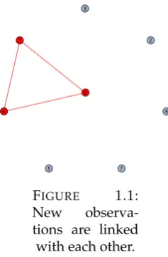
(21) Chapter 1. Dual Decision Processes: Retrieving Preferences when some Choices are Intuitive. 10. that its corresponding environment is not similar enough to any other previous environment. In other words, f (t) ≤ α. Then, any observation s for which the conditional familiarity is less than f (t) must be generated by S2 too. In fact, f (s|as ) ≤ f (t) ≤ α implies that no past behavior that could have been replicated in s comes from an environment that is similar enough to the one in s. Thus, any observation linked with a new observation must be generated by S2. It is easy to see that this reasoning can be iterated, in fact, any observation linked with an observation generated by S2 must be generated by S2 too. Similarly, consider a least novel observation in a cycle t, that we know is generated by S1. Any observation s for which the unconditional familiarity is greater than the conditional familiarity of t must be generated by S1 too. In fact, we know that α < f (t|at ) because t is generated by S1. Then, any observation s to which t is linked has an unconditional familiarity above α, which implies that some past behavior could be replicated by S1, and so such observation must be generated by S1 too. Again, the reasoning can be iterated. Thus, we can start from a small subset of observations undoubtedly generated by either S1 or S2, inferring from there which other observations are of the same type. We now use Example 1 to illustrate the algorithm. In doing so, we show that it is possible to see our algorithmic analysis in terms of graph theory. In fact, when two observations are linked we can think of them as connected by an undirected edge. Then, we can clearly see that DN and DC have to be the sets containing all those nodes that belong to the connected components of new and least novel observations in a cycle respectively. Graphical Intuition: Example 1 Suppose that we observe the decisions made by the DM in Example 1, without any knowledge on his preferences or similarity threshold α. The following table summarizes the different observations. t=1 3, 4, 5, 6 a1 = 3. t=2 1, 2, 3, 4, 5, 6 a2 = 3. t=3 1, 3, 4, 7 a3 = 1. t=4 2, 4, 7 a4 = 2. t=5 1, 3, 6 a5 = 1. t=6 1, 2, 3, 4 a6 = 1. t=7 2, 4, 8 a7 = 2. t=8 2, 4, 8, 9, 10 a8 = 2. We can easily see that the only new observations are observations 1, 3 and 4, and hence we can directly infer that S2 was active in making the corresponding choices. It is immediate to see that new observations are always linked to each other and hence, observations 1, 3 and 4 are connected by undirected edges as in the graph of Figure 1.1.22 22. Notice that for any new observation t, f (t|at ) = 0..

(22) 1.4. The Revealed Preference Analysis of Dual Decisions. 11. 8. 1. 2. 3. 4. 6. 5. 7. F IGURE 1.1: New observations are linked with each other.. We can go one step further and consider observation 5. From observed behavior we cannot understand whether the choice comes from maximization of preferences or the replication of past behavior in period 3. Nevertheless, S2 was active in period 3 and one can easily see that f (5|a5 ) = 25 ≤ 37 = f (3), making observation 5 linked with observation 3 and according to Proposition 1, making it generated by S2 too. This is represented in Figure 1.2. 8. 1. 2. 3. 4. 6. 5. 7. F IGURE 1.2: 5 is linked with 3. Consider now observation 7. We cannot directly link observation 7 to either observations 1, 3 or 4, because f (7|a7 ) = 21 > max{f (1), f (3), f (4)}. However, we can indirectly link observation 7 to observation 3 through observation 5, because f (7|a7 ) = 12 ≤ 12 = f (5), thus making 7 an element of DN . See Figure 1.3 for a graphical description. No other observation is indirectly linked to observations 1, 3 or 4 and hence, DN = {1, 3, 4, 5, 7}. The method rightfully excludes all S1 observations from DN ..

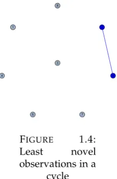
(23) 12. Chapter 1. Dual Decision Processes: Retrieving Preferences when some Choices are Intuitive 8. 1. 2. 3. 4. 6. 5. 7. F IGURE 1.3: 7 is (indirectly) linked with (3) 5. The example presents inconsistencies in the revealed preference. Observation 3 and 6 are both in conflict with observation 2. That is, observations 2 and 3 and 2 and 6 form cycles. Then, noticing that max{f (2), f (3)} = f (2) and that max{f (2), f (6)} = f (2) = f (6) we can say that observations 2 and 6 are generated by S1 thanks to Proposition 1, given they are least novel in a cycle. It is immediate again to see that 2 and 6 are connected by an undirected edge. See Figure 1.4 for a graphical description. 8. 1. 2. 3. 4. 6. 5. 7. F IGURE 1.4: Least novel observations in a cycle. But then, notice that observation 6 is linked to observation 8 given that f (6|a6 ) = ≤ f (8) = 35 revealing that the latter must have been generated by S1 too. Figure 1.5 shows this idea graphically. Thus, we get DC = {2, 6, 8} that were the observations rightfully excluded from DN . No decision made by S2 has been cataloged as intuitive. Thanks to the algorithm, we found the two connected components as shown in Figure 1.6. 3 5.

(24) 1.5. A Characterization of Dual Decision Processes. 8. 8. 1. 2. 1. 2. 3. 3. 4. 6. 5. 13. 4. 6. 7. 5. F IGURE 1.5: 6 is linked with 8. 7. F IGURE 1.6: DN and DC .. The modified revealed preference exercise helps us determine that alternative 1 is better than any alternative from 2 to 7, alternative 3 is better than any alternative from 4 to 6, and alternative 2 is better than alternatives 4, 7 and 8 as it is indeed the case. The value of the similarity threshold α by Proposition 1 can be correctly determined to be in the interval [0.5, 0.6) thanks to the information retrieved from observations 7 and 8 respectively. Notice that in general DN and DC will be proper subsets of the whole S2 and S1 sets of observations, respectively. The set DN is built upon the set of new observations and those indirectly linked to them.23 It may be the case that some S2 observations are not linked to other S2 observations.24 Nonetheless, if the observations are rich enough, it is possible to guarantee that DN and DC coincide with the sets of conscious and intuitive decisions. In the following section we analyze a rich dataset, where richness is achieved through social data, that allows for the identification of the two sets of conscious and intuitive observations.25 More importantly, notice that Proposition 1 relies on one important assumption, that is, the collection of observations is generated by a DD process. The following section addresses this issue.. 1.5. A Characterization of Dual Decision Processes. In section 1.4 we showed how to elicit the preferences and the similarity threshold of an individual that follows a DD process. Here, building upon the results of that section, we provide a necessary and sufficient condition for a set of observations to be characterized as a DD process with a known similarity function. In other words, we provide a condition that can be used to falsify our model. Finally, we provide an alternative characterization of the model whenever the similarity function is also unknown and observations generated by an homogeneous population are available. This alternative characterization allows us to uniquely identify the preferences of the DM and also how similarity comparisons are made. 23. DN is never empty because it always contains the first observation. For this reason, nothing guarantees that D \ DN are intuitive observations and hence, Proposition 1 needs to show how to dually construct a set of intuitive decisions DC . 25 In section 1.6 we study the case of a forgetful decision maker and we show how in such case it is possible to identify the two sets when one sequence of observations is rich enough. 24.

(25) 14. Chapter 1. Dual Decision Processes: Retrieving Preferences when some Choices are Intuitive. From the construction of the set DN , we understand that a necessary condition for a dataset to be generated by a DD process is that the indirect revealed preference we obtain from observations in DN , i.e. R(DN ), must be asymmetric. It turns out that this condition is not only necessary but also sufficient to represent a sequence of decision problems as if generated by a DD process. One simple postulate of choice characterizes the whole class of DD processes. Interestingly enough though, it is possible to characterize such class with a condition that is computationally easier to test. Axiom 1 (Link-Consistency) A sequence of observations {(At , et , at )}Tt=1 satisfies Link-Consistency if, for every t ∈ DN , xR(t)y implies not yR(L(t))x. This is a weakening of the Strong Axiom of Revealed Preference. In fact it imposes that no cycle can be observed when looking at an observation t in DN and those directly linked to it. This condition is easy to test computationally because it only asks to check for acyclicity between linked observations. The next theorem shows that such condition is indeed necessary and sufficient to characterize DD processes with known similarity. Theorem 1 A sequence of observations {(At , et , at )}Tt=1 satisfies Link-Consistency if and only if there exist a preference relation and a similarity threshold α that characterize a DD process. The theorem is saying that Link-Consistency makes possible to determine whether the DM is following a DD process or not. In particular, when the property is satisfied, we can characterize the preferences of the DM with a completion of R(DN ) which is asymmetric thanks to Link-Consistency and use the lower bound of α as described in Proposition 1 to characterize the similarity threshold. In fact, by construction, for any observation t outside DN it is possible to find a preceding observation that can be replicated, i.e. the one defining f (t|at ). Clearly the familiarity of an observation can be defined only if the similarity function is known. In the final part of this section we show how to identify such function from a population of heterogeneous individuals following a DD process. Here we propose an alternative approach, that also uses social data, that allows us to jointly determine preferences and similarity comparisons. Notice that we do not assume any particular structure for the sequence of observations we use as data and hence, the characterization of preferences does not have to be unique, even when the similarity is known. One way to uniquely characterize the preferences of the DM that allow us also to determine how similarity comparisons are made, is to get different sequences of observations generated by an homogeneous population. That is, suppose we observe many and different sequences of decision problems and choices generated by a population of individuals sharing the same preferences, similarity threshold and similarity function.26 Let D be the set containing such sequences and D ∈ D be the collection of observations composing one of them. Then, if D is rich enough we can perfectly identify not only the preference relation but also, for every decision environment, which other environments are considered similar enough and which are 26 It is possible to argue that individuals that share the same socioeconomic characteristics and have similar cognitive capabilities are likely to be described by the same DD process..

(26) 1.5. A Characterization of Dual Decision Processes. 15. not. Notice that this completely identifies the model. In fact, the similarity threshold and the similarity function define a binary similarity function, i.e. a Boolean similarity function. That is, given any environment, the combination of similarity function and similarity threshold partitions the set of environments in two sets of similar and dissimilar environments. Thus, knowing for every decision environment which other environments are considered similar enough and which are not, completely identifies such function. We say that D is rich if: • for any x, y ∈ X there exists a D ∈ D such that there is some t ∈ D where x, y 6= as for s < t and At = {x, y}. • for any x, y, z ∈ X there exists a D ∈ D such that there is some t ∈ D where x, y, z 6= as for s < t and At = {x, y, z}. • for any e, e0 ∈ E and any x, y ∈ X, there exists a D ∈ D such that there is some t ∈ D where x, y 6= as for s < t − 1 and At−1 = {y}, et−1 = e0 , At = {x, y} and et = e. The first two requirements impose that for every pair and triple of alternatives, there is some collection D in which until some moment in time t, they have never been chosen.27 That is, for any pair and triples of alternatives there is a sequence of decision problems in which for some moment in time t they were part of a new observation. The third requirement imposes that for any pair of environments and any pair of alternatives there is a sequence of observations such that the environments are part of two consecutive decision problems in which the two alternatives have never been chosen before. Thus, the choice in t can be either new or the same as in t−1. These conditions allow us to perfectly identify the preferences of the homogeneous population and how analogies are made whenever the observed choices satisfy some consistency requirements. Before stating such requirements, it is useful to define a set for any environment e ∈ E that contains all those environments that would be considered similar enough to e by a DM following a DD process. Suppose, without loss of generality, that for some D ∈ D there exists t ∈ D such that At = {x, y} and at = x with x, y 6= as for s < t. If the observations are generated by a DM following a DD process, then t would be a new observation and x would be revealed preferred to y. Then let S(e) be defined as follows: S(e) = {e0 ∈ E| ∃D ∈ D such that, for some t ∈ D, t − 1 = ({y}, e0 , y) is new and t = ({x, y}, e, y)}.. For the same reasoning developed before, if the observations are generated by individuals following a DD process, S(e) would contain only environments considered similar enough to e because the observed inversion of preferences in t is possible only when past behavior is replicated. In fact, if y is chosen over x in t, it must be because of replication of behavior in t − 1. This is a concept similar to the one of revealed preferences. Environment e0 is revealed similar to e whenever such inversion of preferences occurs. Notice that by richness, S(e) would contain all those environments that are considered similar enough to e. 27. Notice that the first two conditions play the same role of the Universal Domain assumption in standard choice theory..

(27) Chapter 1. Dual Decision Processes: Retrieving Preferences when some Choices are Intuitive. 16. Finally, for any collection D ∈ D define for all observations t ∈ D the following set: I(t) = {x ∈ X| x = as , for some s < t such that as ∈ At and es ∈ S(et )}. If the observations are generated by DD processes, I(t) would contain all those past choices that could be replicated in t. Now we have all the ingredients to state the consistency requirements that characterize the whole class of DD processes for a rich dataset D. The following axioms are intended for D, D0 ∈ D. The first axiom requires that conscious choices are consistent. That is, there do not exist two observations in which x is consciously chosen over y in one of them and y over x in the other. This is a weakening of the Weak Axiom of Revealed Preference (WARP). Axiom 2 (Conscious Consistency (CC)) For any t ∈ D and t0 ∈ D0 such that I(t) = I(t0 ) = ∅, if x, y ∈ At ∩ At0 and x = at then y 6= at0 . The second axiom requires that intuitive choices come from replication of past behavior. Axiom 3 (Intuitive Consistency (IC)) For any t ∈ D such that I(t) 6= ∅, at ∈ I(t). Then we can state the following theorem. Theorem 2 A rich dataset D satisfies CC and IC if and only if there exist a preference relation , a similarity function σ and a similarity threshold α that characterize a DD process. Moreover, the preference relation and the binary similarity function defined by σ and α are uniquely identified. Intuitively, the first two requirements of a rich dataset plus CC assure that the revealed preference relation constructed from the observations that would have to be explained as conscious choices is complete and transitive. Then, IC assures that those choices that should be explained as intuitive, replicate past behavior. Uniqueness comes from the fact that every pairwise comparison between alternatives and between environments is observable thanks to richness.. 1.5.1. On Conscious and Intuitive Behavior. Throughout all the chapter we have assumed that conscious behavior is the maximization of a given preference relation. In some cases this assumption can be too strong. The framework we propose does not depend on the particular conscious behavior that is assumed. In fact, as the previous analysis should clarify, for any given decision environment analogies determine a partition with two components, one containing those problems that are similar enough to the reference environment and another one containing those that are not. Such partition is based only on one and simple assumption, intuitive behavior must come from the replication of past behavior. Alternative conscious behaviors are possible, the only element of the formal analysis we conducted that has to be changed is what kind of consistency requirement to test on those problems that fall in the part of the.

(28) 1.5. A Characterization of Dual Decision Processes. 17. partition that has to be assigned to conscious behavior.28 Thus we can think about preferences that depend on the decision environment or preferences that satisfy only quasi-transitivity or less consistent choice behaviors that are falsifiable and we would still be able to run the same kind of analysis. The purpose of this kind of flexible framework is to provide a theoretical benchmark to analyze in a structured way what conscious and intuitive behavior are. The model we propose here is just a first step into this new direction and hence it is simplified to keep the analysis focused on the novel aspect of the problem we address, that is, (i) the relationship between intuitive and conscious choices and (ii) the structure observed behavior should have once we consider these two sources of individual behavior. Finally, notice that the assumptions that intuitive behavior comes from the replication of past behavior is much less restrictive than what would appear at a first glance. We have considered only the case of replicating past choices made by the same DM because we are considering a fictitious and quite restrictive decision theoretic environment. It would be easy to incorporate social considerations by changing what experiences and decision problems form part of the DM’s memory. For example, we can consider cases where the DM stores in his memory not only his experiences, but also his parents’, siblings’ or friends’ experiences thus making the concept more general than what the literal interpretation of the model would suggest.. 1.5.2. Estimation of the Similarity Function. The similarity function is a key component of a DD process and for the sake of exposition it is assumed to be known in the main part of the chapter. Nonetheless, we discuss here how to identify it by studying the choice behavior of a group of individuals sharing it. Consider a continuous population of individuals sharing the similarity function σ, with a continuous and independent distribution of the similarity threshold over [0, 1]. Sequences of decision problems and preferences are independently distributed. Consider a pair of alternatives x, y ∈ X such that each of them is considered better than the other for a non-negligible part of the population. For every pair of environments e, e0 ∈ E, assume there exists a non-negligible subpopulation for which there is an observation t as follows: • x 6∈ At , At+1 = At ∪ {x} and no alternative in At+1 was chosen before t, • et = e0 and et+1 = e and • at = y. The main result of this section shows that we can compare the similarity of two different pairs of environments by considering the corresponding aforementioned subpopulations and sampling them. Formally, denote by ν(e, e0 ) the average relative number of randomly sampled individuals sticking to y at t + 1. That is, for any pair of environments (e, e0 ) we take a sample of finite magnitude n from the aforementioned subpopulations and 28 Obviously, dually, to find intuitive choices we should analyze violations of such requirements..

(29) 18. Chapter 1. Dual Decision Processes: Retrieving Preferences when some Choices are Intuitive. we compute the average of the relative number of individuals that stick to y in such sample. Such average is ν(e, e0 ). Proposition 2 (Eliciting the Similarity) For every two pairs of environments p (e, e0 ) and (g, g 0 ), P r(ν(e, e0 ) ≥ ν(g, g 0 )|σ(g, g 0 ) > σ(e, e0 )) → 0. That is, the probability of having ν(e, e0 ) ≥ ν(g, g 0 ) when σ(g, g 0 ) > σ(e, e0 ) probabilistically converges to zero. Given our assumptions, each sample we take to calculate ν(e, e0 ) is an independent estimation of the relative number of individuals that sticks to y. Thus, we are getting a consistent estimate of the relative number of individuals that would stick to y in the whole subpopulation. Then, comparing the average relative number of individuals that stick to alternative y in t + 1 for different pairs of environments, gives the required information on the similarity function. The main intuition of Proposition 2 is the following. There are two reasons that force the average relative number of people sticking to y with the pair of environments (e, e0 ) to be bigger than the average relative number of people sticking to y with another pair of environments (g, g 0 ). First, the pair of environments (e, e0 ) is more similar than the pair of environments (g, g 0 ). This implies that S1 is active in t + 1 for a larger number of individuals on average, which leads to replication of the choice in t, i.e. alternative y.29 Second, y is preferred to x by a larger number of sampled people among those using S2 with the pair of environments (e, e0 ). The law of large numbers makes the second concern disappear as the number of samples taken to measure ν grows, revealing the similarity of different pairs of environments.. 1.6. Extensions. The analysis developed in the previous sections is based on two assumptions that we relax here. First, we have assumed that the DM has perfect memory. In this section we show that such an assumption is not needed to perform the algorithmic analysis. Moreover, if some richness conditions are satisfied by the sequence of decision problems under study, we show that by considering imperfect memory we can completely identify the preferences of the DM and determine which system generated every single observation by studying just one sequence of observations. The second assumption we relax concerns the similarity function. We show that the analysis of the previous sections is perfectly valid, even if we have only partial information regarding the similarity function.. 1.6.1. A Forgetful Decision Maker. So far, we have assumed that the DM has perfect memory, i.e. intuitive decisions can come from the replication of any past choice. In this section, we depart from such assumption and analyze the possibility of a DM that forgets older choices. 29 Notice that our assumptions imply that only the choice in t can be replicated if S1 is active..