A New Strategy for Adapting the Mutation Probability
in Genetic Algorithms
Natalia Stark, Gabriela Minetti, Carolina Salto
Laboratorio de Investigación en Sistemas Inteligentes Facultad de Ingeniería – UNLPam
Calle 110 N°390 – General Pico – La Pampa Email: {nstark,minettig,saltoc}@ing.unlpam.edu.ar
Abstract.
Traditionally in Genetic Algorithms, the mutation probability parameter maintains a constant value during the search. However, an important difficulty is to determine a priori which probability value is the best suited for a given problem. Besides, there is a growing demand for up-to-date optimization software, applicable by a non-specialist within an industrial development environment. These issues encourage us to propose an adaptive evolutionary algorithm that includes a mechanism to modify the mutation probability without external control. This process of dynamic adaptation happens while the algorithm is searching for the problem solution. This eliminates a very expensive computational phase related to the pre-tuning of the algorithmic parameters. We compare the performance of our adaptive proposal against traditional genetic algorithms with fixed parameter values in a numerical way. The empirical comparisons, over a range of NK-Landscapes instances, show that a genetic algorithm incorporating a strategy for adapting the mutation probability outperforms the same algorithm using fixed mutation rates.
1.
Introduction
During the design process of a Genetic Algorithm (GA), we need to instantiate several parameters to specific values before the run of the algorithm, in order to obtain a robust search technique. This task is also known as pre-tuning of algorithmic parameters. There are at least two possible approaches to determine the optimal value of the parameters to use beforethe GA is initiated: parametertuning and parametercontrol
[11]. The first one is related to make an extensive experimentation to determine, in an empirical way, which parameter values actually give the best results for the problem at hand; this task implies an extra set up time, which is computationally expensive and rarely reported in the literature. In this sense, several approaches have been reported in the literature, such us Design of Experiments [20], F-RACE [7], and REVAC [19]. The second approach consists in doing changes in the parameter values during a GA run. This requires initial parameter values and suitable control strategies, which in turn can be deterministic, adaptive or self-adaptive. These strategies manage information that influence the parameter values during the search and define a set of criteria to produce changes. Our proposal follows an adaptive approach, which the most important precedent is found in [9]. However, many relevant approaches have been proposed for adjusting GA parameters such as genetic operator probabilities [17,24,25,26], selection methods [6,13], population size [4,12,23,28] in the course of a genetic algorithm run.
Among the GA parameters, we can mention the mutation probability (pm) as a critical parameter to its
performance. Large values of pm transform the GA into a purely random search algorithm, while some
mutation is required to prevent the premature convergence of the GA to suboptimal solutions. Many different fixed mutation probabilities for GAs have been suggested in the literature, which are derived from experience o by trial-and-error. De Jong proposed pm=0.001 in [9] meanwhile Grefenstette suggested pm=0.01 [14].
According to Schaffer, pm should be set to [0.005, 0.01] [21]. In [5], Bäck proposed pm=1.75/(μ *L1/2), where
μ indicates the population size and L denotes the length of individuals. In [18], it is suggested that pm=1/L
should be generally “optimal”. It is very difficult, though not impossible, to find an appropriate parameter setting for pm in order to reach an optimal performance.
behaviour of the GA, avoiding the premature convergence and lost of genetic diversity. Moreover, this method is implemented without introducing any major changes to its original algorithm design. The algorithm makes decisions during the search based on the current information, by using a control strategy based on the current population entropy. As a consequence, the pm value changes throught the search, based on the
potential advantages that such changes could bring. The adaptation of pm value is important to allow the
search process to optimize its performance during run time. Moreover, it frees the user of the need to make non-trivial decisions beforehand which are a very expensive task. An additional benefit of our adaptive strategy is the reduction in the time related to the pre-tuning phase, because the mutation probability value does not need to be tuned.
Researchers from the metaheuristics community have also been motivated on this subject proposing methods for control the mutation probability, using different statistics from the current state of the search to make their decisions. For instance, Thierens [27] recently proposed an adaptive mutation rate control approaches based on the stochastic Manhattan learning algorithm. A recent research from Montero et al. [17] proposed an adaptive approach for the genetic operator probabilities based on penalties and rewards, considering the information of the operator performance in the last l previous generations. Blum et al. [8] introduced a method of adapting mutation parameters based on the fitness frequency distribution, to determine the current search state, and another that evaluates successful mutations and modulates probability density functions of mutation steps. In order to prevent the premature convergence, Zai-jian [29] analysed the drawbacks of the traditional mutation operator and presented a mutation operator based on information entropy, that replaces it.
The performance of our proposed algorithm will be evaluated using the NK model [15]. This problem provides a tuneable set of landscapes with increasing numbers of optima and decreasing fitness correlations as
K is increased. NK-Landscapes have been the center of several theoretical and empirical studies both for the statistical properties of the generated landscapes and for their GA-hardness [1, 10].
The outline of the paper is as follows. Section 2 presents the outline of the current implementation of our adaptive algorithm. In Section 3, addresses the optimization problem used. In Section 4, we present the algorithmic parameterization. In the next section, we analyze the results from a numerical point of view. Finally, we summarize the conclusions and discuss several lines for future research in Section 6.
2.
Our Adaptive Proposal
In this section, we present the characteristics of the Adaptive Mutation Probability Genetic Algorithm (APmGA) devised, which dynamically adjusts the mutation probability during the evolutionary process (see the structure of the proposed approach in Algorithm 1). The algorithm creates an initial population P of μ solutions in a random way, and then evaluates these solutions. After that, the population goes into a cycle where it undertakes evolution, which means the application of stochastic operators such as selection, recombination, and mutation to compute a whole generation of new λ individuals. The new population is built up by selecting μnon-repeated individuals from the set of (μ+λ)existing ones. After that, each iteration ends
Algorithm 1 APmGA()
t = 0; {current generation} initialize(P(t));
evaluate(P(t));
while{(t < maxgenerations) do
P'(t) = selection(P(t)); P'(t) = recombinate(P'(t)); P'(t) = mutate(P'(t), pm); evaluate (P'(t));
P(t+1) = Replace(P'(t) ∪ P(t));
(ΔHk,ΔHk-1,pm)=Statistics(P(t+1));
if (t % epoch == 0) then
AdaptivePmControl(ΔHk,ΔHk-1,pm);
t = t + 1; end while
with the computation of the statistics of the current population and the application of the adaptive mechanism to dynamically set the mutation probability, which are described in following paragraphs. Finally, the best solution is identified as the best individual ever found that maximizes the fitness function.
The objective of our adaptive strategy is to increase pm if the genetic diversity is gradually lost in order to
maintain a population distributed in the search space. Otherwise, the pm value is reduced when an increase in
the population diversity is observed. Therefore, these changes in the pm value are also an additional source for
a good balance between exploration and exploitation, intrinsic to the adaptive criterion.
Furthermore, this strategy monitors the genotypic diversity present in the population using the Shannon entropy metric [22], following the ideas presented in [2]. When the entropy value is closed to 0, the population contains identical individuals; otherwise it is positive and maximal when all the individuals in the population are different.
The strategy control uses the population entropy at the end of each epoch (a certain number of consecutive generations). Then it computes the variation of the current entropy at the k epoch (Hk) and entropy from the
previous k-1 epoch (Hk-1), denoted as ΔHk= Hk - Hk-1. This variation, ΔHk, is compared with the one observed
in previous epoch (ΔHk-1= Hk-1 - Hk-2), as shown in Algorithm 2. In this way, when the entropic variations
decrease at least in a factor of ε indicate lost of diversity, in a consequence the mutation probability value will be changed by adding a constant factor (α). Otherwise, the pm value is decreased by subtracting the α
value. In order to prevent the overshooting of pm, this algorithm controls that pm belongs to [pmLB, pmUB];
where the lower bound of pm is pmLB =0.001 and the upper bound is pmUB =0.1. These bounds are selected
taking into the account the values suggested in literature, as mention in Section 1.
The algorithm policy in APmGA is different from all approaches described above. In [27], the authors use a different criterion to modify pm based on stochastic Manhattan learning algorithm. APmGA is different from
[17] because we do not use a policy of penalty and rewards. In [8], pm is varied considering the fitness
frequency distribution. Finally, Zai-jian [29] uses the entropy value to modify the mutation operator instead of the probability mutation values as we did in this work.
3.
NK-Landscapes
An NK-Landscape is a fitness function f : { 0,1 }N→ R on binary strings, where N is the bit string length and K is the number of bits in the string that epistatically interact with each bit, i.e., K stands for the number of other genes that epistatically affect the contribution of each gene to the overall fitness value of the string. Each gene xi, where 1 = xi = N, contributes to the total fitness of the genotype depending on the value of its
allele and on those of each of the K other genes to which it is linked. Thus K must fall between 0 and N-1. For
K = 0, there are no interaction among genes and a single-peak landscape is obtained; in the other extreme (for
K= N-1), all genes interact each other in constructing the fitness landscape, so a completely random landscape is obtained (a maximally rugged landscape). Varying K from 0 to N-1 gives a family of increasingly rugged multi-peaked landscapes.
Algorithm 2 AdaptivePmControl(ΔHk, ΔHk-1,pm) function
{Adapt the pm value} if ΔHk < (1+ε).ΔHk-1 then pm= pm+α
else
pm= pm-α
{Maintain pm in the range [pmLB,pmUB]} if pm < pmLB then
pm= pmLB
else if pm > pmUB then
The fitness value for the entire genotype is given as the average of the fitness contribution of each locus fi
by:
∑
== N
i fi xi xi xiK
N x f
1 ( , , )
1 ) (
1 K
(1)
where
{
}
K i
i x
x ,K
1 ⊂
{
x1,Kxi−1,xi+1,K,xN}
are the K genes interacting with gene xiin the genotype x. Theother K epistatic genes could be chosen in any number of ways from the N genes in the genotype. Kauffman [16] investigated two possibilities: adjacent neighborhoods, where K genes nearest to gene xi on the
chromosome are chosen, particularly a gene interacts with K/2 left and K/2 right adjacent genes; and random neighborhoods, where these K other genes are chosen randomly on the chromosome. In this work we adopted the first type of neighbourhood and considered circular genotypes to avoid boundary effects. The fitness contribution fiof xi is taken at random from a uniform distribution [0.0, 1.0] and depends upon its value and
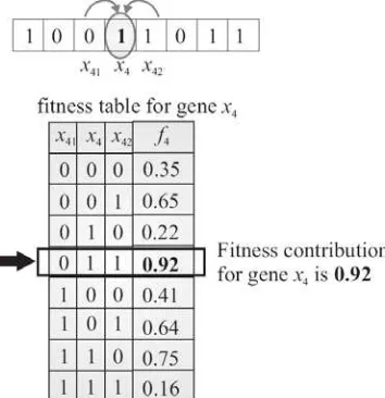
those present in K other genes among the N. Each gene has associated a fitness table, mapping each of the 2K+1 possible combinations of alleles to a random, real value number in the range [0,1]. Fig. 1 gives an example of the fitness function function f4
(
x4,x41,x42)
associated to gene x4 for N=8 and K=2. Gene x4 islinked to two other genes, in this case, the gene to both sides,
1 4
x and
2 4
[image:4.612.239.416.289.472.2]x .
Fig. 1. An example of a genotype and a fitness table associated to gene x4 for a problem with N=8 and K=2.
4.
Experimental Setup
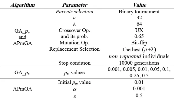
In order to observe and compare the effect on performance of our adaptive GA, we use a GA with fixed mutation probability. For comparison purposes, we use six different mutation probability values for the GA, ranging from 0.005 to 0.5, i.e from very low to very high probabilities values. We denote the GA variants as GA_pm, for example: GA_0.05 is a GA using a mutation probability equal to 0.05.
Table 1. Parametric values used for the different GAs
Algorithm Parameter Value
Parents selection
μ Binary tournament 32
λ 64
Crossover Op. and its prob.
UX 0.65 Mutation Op.
Replacement Selection
Bit-flip The best (μ+λ) non-repeated individuals GA_pm
and APmGA
Stop condition 10000 generations
GA_pm pm values
0.001, 0.005, 0.01, 0.05, 0.1, 0.25, 0.5
Initial pm value 0.01
α 0.001
APmGA
ε 0.5
We conduct our study on NK instances with N=96 bits varying the epistatic relations from K=0 to K=48 in increments of 4, adding up to 13 instances. We use landscapes with adjacent epistatic patterns among genes. For each combination of N and K we generated 30 random problem instances.
The algorithms are implemented inside MALLBA [3], a C++ software library fostering rapid prototyping of hybrid and parallel algorithms. Our computing system is a cluster of 8 machines with AMD Phenom8450 Triple-core Processor at 2GHz with 2 GB of RAM, linked by Gigabit, under Linux with 2.6.27-4GB kernel version.
In order to get concluding results from the comparison made, we have performed some statistical tests on the results. Before performing the statistical tests, we first check whether the data follow a normal distribution by applying the Shapiro-Wilks test. When the data are normally distributed, we perform an ANOVA test. Otherwise, the tool we use is the Kruskal-Wallis test. This statistical study allows us to asses if there are meaningful differences among the compared algorithms with 95% confidence level.
5.
Experimental Results
In this section, we compare the performance of APmGA against the GA variants. Our aim is to offer an analysis from the accuracy (quality) and performance points of view. For this purpose, this section consists of two parts. First, we analyze the solutions quality obtained by the studied algorithms. In the second part, we study the computational effort of each algorithm.
5.1. Analysis of the Algorithmic Behavior Considering the Quality Solutions
In order to evaluate the quality of solutions, we begin showing the effect of mutation probability on the performance of GA variants and APmGA. The Fig. 2 plots the best solutions observed over the 30 runs for each K value and each algorithm. From this figure, we can see that using small pm values (in the range
[0.01..0.001]) allows the GA to find higher solutions than GA variants. APmGA also obtains promising solutions for the majority of the instances: in 11 of the 13 instances outperforms both GA_0.01 and GA_0.001, meanwhile in 8 of the 13 instances to GA_0.005. The reason for this quality improvement is due to that APmGA adapts the pm keeping it at very low values (pm < 0.01).
In the following, we compare the APmGA solutions against the ones of the GA variants by using the percentage gap. This measure is the relative distance to the average of the best solutions obtained by APmGA (best_solAPmGA) and the average of the best solutions found by the GAs variants, as described in Equation 2.
100 _
_
_ − ×
=
APmGA m APmGA
sol best
p GA sol
best
0.64 0.66 0.68 0.70 0.72 0.74 0.76 0.78 0.80
0 4 8 12 16 20 24 28 32 36 40 44 48
K
co
st
[image:6.612.146.484.77.295.2]GA_0.001 GA_0.005 GA_0.01 GA_0.05 GA_0.1 GA_0.25 GA_0.5 APmGA
Fig. 2. Best values for each algorithm
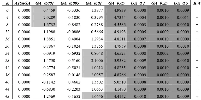
Hence, Table 2 shows the gap values of each GA variants on each problem instance. Positive values indicate superiority of the results obtained by the proposed APmGA, while negative values indicate the opposite condition. Additionally, we show the results of the statistical tests in the comparison of the different algorithms for each tested instance in the last column. Symbol ’+’ means that significant differences where found at 95% confidentiality, and cells with distinct backgrounds in the same row means the respective GA variants behave statically different for the given instance. For example, in the last row (K=48), we see that the APmGA, GA_0.001 and GA_0.005 are similar among them and different from the remaining GA variants.
As we can see in Table 2, APmGA outperforms the GA variants with pm≥ 0.01 for all instances, except
GA_0.01 for K=4. Comparing the APmGA with GA_0.001, we observe positive gaps in 10 of 13 instances. The worst APmGA performance is detected when it is compared with GA_0.005. However, in general the APmGA performance is statistically similar to the performance of the GA variants with pm ≤ 0.01 (white
Table 2. Gap values for GA-pm
K APmGA GA_0.001 GA_0.005 GA_0.01 GA_0.05 GA_0.1 GA_0.25 GA_0.5 KW
0 0.0000 0.4459 -0.3336 1.3977 4.9839 0.0008 0.0010 0.0009 +
4 0.0000 2.0289 -0.1830 -0.3995 4.7354 0.0004 0.0010 0.0011 +
8 0.0000 1.6732 -0.8482 0.2738 4.5586 0.0003 0.0010 0.0010 +
12 0.0000 1.1988 -0.0886 0.5666 4.9198 0.0005 0.0009 0.0009 +
16 0.0000 1.8851 0.4904 1.2934 4.8211 0.0007 0.0010 0.0009 +
20 0.0000 0.7867 -0.1024 1.3855 4.7959 0.0008 0.0010 0.0010 +
24 0.0000 0.0919 -0.6932 0.8048 4.6523 0.0008 0.0009 0.0009 +
28 0.0000 1.4750 0.5160 2.1006 5.9582 0.0009 0.0010 0.0010 +
32 0.0000 0.2774 -0.5021 1.0212 4.8235 0.0009 0.0010 0.0010 +
36 0.0000 0.2587 0.0148 2.0957 4.8766 0.0009 0.0009 0.0009 +
40 0.0000 -0.1142 0.4662 1.3502 5.0510 0.0008 0.0010 0.0009 +
44 0.0000 -0.6830 -0.2203 1.0653 4.1470 0.0009 0.0010 0.0009 +
[image:6.612.92.511.499.708.2]background). Furthermore, these variants and APmGA outperforms the remaining GAs with fixed pm≥ 0.05
(grayscale background). This suggests that the best behaviour of a GA for this kind of problem is obtained when the mutation probability is very low. This means that our adaptive strategy makes appropriate changes in the pm value in order to obtain high quality solutions. Another issue to emphasize is that the adaptive
approach implicitly helps in minimizing the work involved in the selection of the appropriate mutation rate to solve the problem.
5.1. Analysis of the Algorithmic Behavior Considering the Computational Effort
Regarding the convergence velocity, Fig. 3 shows the mean number of generations for each algorithm. Each bar corresponds to the average of mean number of generations to reach the best value for each instance, averaged over the 30 independent runs. We can see that APmGA needs more numerical effort than GA variants. However, the statistical tests performed indicate that the differences among the algorithms are not significant. As a consequence, the proposed adaptive GA not only computes accurate solutions with high fitness values, but also exhibits a similar convergence velocity than the GA variants with fixed mutation probability during the evolution.
[image:7.612.95.297.280.430.2]0 1000 2000 3000 4000 5000 6000 GA _0.0 1 GA_ 0.05 GA_0 .001 GA_ 0.0 05 GA_0 .1 GA_ 0.25 GA_0 .5 APm GA g e ne ra ti on s 0.00 2.00 4.00 6.00 8.00 10.00 12.00 14.00 GA_0 .005 GA_0. 01 GA_0. 05 GA_0. 1 GA _0.25 GA _0. 5 AP mG A ti me ( m in u te s )
Fig. 3. Mean number of generations for each
algorithm Fig. 4. Mean time by execution for each algorithm
Finally, we analyze the GA variants and APmGA behaviors considering the execution time. If we examine the average amount of time necessary to execute the algorithms in Fig. 4, we can see that APmGA presents similar execution times than the majority of the GA variants. The previous observation suggests that our proposal does not add significant computational time to compute the Shannon entropy at the end of each epoch, which is the base of our control strategy. The statistical tests have provided these results with 95% confidence level.
A remarkable point here is that our proposal provides an additional source of time savings, since we avoid the pre-tuning phase of one parameter of the algorithm. Indeed, APmGA needs 75 hours of execution to obtain the results from the 30 independent executions for the entire set of instances addressed in this work (13 instances). For the GA variants, seven values have been considered for the mutation probability. Let us assume it takes 73 hours of computation for each variant, therefore 73 × 7 = 511 hours of computation have been required. This means that APmGA has allowed us to avoid running 6 configurations, thus saving 436 hours of pre-tuning: the time has been reduced by 85%.
[image:7.612.323.517.286.427.2]6.
Conclusions
In this paper, we present an adaptive GA (APmGA) that guides the genetic search using an adaptive strategy to control the mutation probability. This strategy is based on the variations of the population entropy between the current and previous epoch. The main goal of APmGA is to modify the mutation probability value during the evolution without external control, in order to prevent the premature convergence and find high quality solutions. Furthermore, this proposal reduces the pre-tuning time to determinate the most appropriate mutation probability value to enhance the algorithm performance.
The results obtained by our adaptive algorithm are very encouraging, since it can obtain high quality solutions than any GA variants with fixed mutation probabilities, and also exhibits a similar convergence velocity. An important remark is that our proposal does not add significant computational time by applying the control strategy to adapt the mutation probability values. Finally, as the APmGA dynamically determines the mutation rate during the search, this adaptive method helps to alleviate the setting time required, by at least 85%, to determine the best mutation rate in traditional GAs, which implies a costly exploration.
As a future work, we propose to study more sophisticated criteria for the adaptation, also possibly including in this process the probability of recombination. Furthermore, another extension to this work can be the analysis of the effectiveness of this adaptive approach over other complex problems.
Acknowledgements
We acknowledge the Universidad Nacional de La Pampa and the ANPCYT (Argentina) from which the authors receive continuous support.
References
[1] H. Aguirre and K. Tanaka. “Genetic algorithms on nk-landscapes: Effects of selection, drift, mutation, and recombination”, EvoWorkshops 2003, LNCS 2611, pp. 131–142, 2003.
[2] E. Alba and B. Dorronsoro, “The Exploration/Exploitation Tradeoff in Dynamic Cellular Genetic Algorithms”, in Procedings of IEEE Transactions on Evolutionary Computation, vol. 9(2), pp. 126-142, 2005.
[3] E. Alba et al. “MALLBA: A Library of Skeletons for Combinatorial Optimisation”, vol. 2400 of LNCS, pp. 927–932, 2002.
[4] J. Arabas, Z. Michalewicz and J. Mulawka, “GAVaPS A genetic algorithm with varying population size”. In Proceedings of the First IEEE Conference on Evolutionary Computation, pp. 73-78, 1994.
[5] T. Bäck. “Self-Adaptation in Genetic Algorithms”. In Proceedings of the 1st European Conference on Artificial Life, pp. 263–271, 1992.
[6] J. E. Baker, “Adaptive selection methods for genetic algorithms,” in Proceedings of the 1st International Conference on Genetic Algorithms and Their Applications, pp. 101–111, 1985.
[7] M. Birattari, T. Stutzle, L. Paquete, and K. Varrentrapp. “A racing algorithm for configuring metaheuristics”. In Proceedings of the 2002 Genetic and Evolutionary Computation Conference, pp. 11–19, 2002.
[8] S. Blum, R. Puisa, J. Riedel, and M. Wintermantel. “Adaptive mutation strategies for evolutionary algorithms”. In The annual conference: EVEN at Weimarer Optimierungsund Stochastiktage 2.0, 2001.
[9] K. A. De Jong, An analysis of the behavior of a class of genetic adaptive systems, Ph.D. dissertation, Univ. of Michigan, Ann Arbor, MI, 1975.
[10] K.A De Jong, M.A. Potter and W.M. Spears, “Using problem generators to explore the effects of epistasis.” In Proceedings of 7th International Conference on Genetic Algorithms, pp. 338-345, 1997
[11] A. E. Eiben, R. Hinterding, and Z. Michalewicz. “Parameter Control in Evolutionary Algorithms”. In IEEE Transactions on Evolutionary Computation., vol. 3(2), pp. 124–141, 1999.
[12] A.E. Eiben E. Marchiori and V.A. Valko. “Evolutionary Algorithms with on-the-fly pop size adjustment”. In Proceedings of Parallel Problem Solving from Nature 2004 (PPSN 2004), vol. 3242 of LNCS , pp.41-50, 2004. [13]A.E. Eiben, M.C. Schut and A.R. de Wilde, “Boosting Genetic Algorithms with Self-Adaptive Selection”, in
Proceedings of the 2006 IEEE Congress on Evolutionary Computation, pp. 16-21, 2006
[14] J. J. Greffenstette. “Optimization of Control Parameters for Genetic Algorithms”. IEEE Transaction on System Man and Cybernetic, vol 16(1), pp. 122–128, 1986.
[16] S. A. Kauffman and S. Levin. “Towards a general theory of adaptive walks on rugged landscapes”. In Journal of Theoretical Biology, vol. 128, pp. 11-45, 1987.
[17] E. Montero and M-C Riff, “On-the-fly calibrating strategies for evolutionary algorithms”, In Information Sciences, vol. 181(3), pp. 552-566, 2011.
[18] H. Mühlenbein. “How Genetic Algorithms Really Work I. Mutation and Hillclimbing”. In Proceedings of the 2nd Conference on Parallel Problem Solving from Nature, pp. 15–29, 1992.
[19] V. Nannen and A. Eiben, “Relevance estimation and value calibration of evolutionary algorithm parameters”. In Proceedings of the Joint International Conference for Artificial Intelligence (IJCAI), pp. 975–980, 2006.
[20] E. Ridge and D. Kudenko. “Tuning an algorithm using design of experiments”. In Experimental Methods for the Analysis of Optimization Algorithms, pp. 265 –286, 2010.
[21] J. D. Schaffer, R. A. Caruana, L.J. Eshelman, R. Das, “A study of control parameters affecting online performance of genetic algorithms for function optimization”, In Proceedings of the third international conference on Genetic algorithms, pp. 51 – 60, 1989.
[22] C.E. Shannon. “A mathematical theory of communication”. In Bell System Technical Journal, vol. 27, pp. 379–423 and 623–656, 1948.
[23] X. H. Shi, L. M. Wan, H. P. Lee, X. W. Yang, L. M. Wang and Y. C. Liang. “An Improved Genetic Algorithm with Variable Population-Size and a PSO-GA Based Hybrid Evolutionary Algorithm.” In Proceedings of the Second International Conference on Machine Learning and Cybernetics, pp. 1735-1740, 2003.
[24] M. Srinivas and L.M. Patnaik, “Adaptive Probabilities of Crossover and Mutation in Genetic Algorithms”. In IEEE Transactions on Systems, Man and Cybernetics, vol. 24 (4), pp. 656-667, 1994.
[25] J.E. Smith and T.C. Fogarty, “Operator and parameter adaptation in genetic algorithms”. In Soft Computing, vol. 1(2), pp. 81–87, 1997.
[26] D. Thierens, “Adaptive strategies for operator allocation”, in Parameter Setting in Evolutionary Algorithms, Springer, pp. 77–90, 2007.
[27] D. Thierens, “Adaptive Mutation Rate Control Schemes in Genetic Algorithms”. In Proceedings of the 2002 IEEE World Congress on Computational Intelligence: Congress on Evolutionary Computation, pp. 980-985, 2002.
[28] D. Voosen and H. Mülhenbein, “Adaptation population size by competing subpopulations”. In Proceedings of the 1996 IEEE Conference on Evolutionary Computation, pp. 330-335, 1996.