A Stand Density Management Diagram for mixed stands of Pinus sylvestris and Pinus pinaster in the Sierra de la Demanda (Spain)

Master Erasmus Mundus in

Mediterranean Forestry and Natural Resources

(MEDFOR)

A Stand Density Management Diagram

for mixed stands of Pinus sylvestris and

Pinus pinaster in the Sierra de la

Demanda (Spain)

Student: Ali Askarieh

Co-advisors: Dr. Irene Ruano Benito, & Prof. Dr. Felipe Bravo Oviedo

INDEX

RESUMEN ... 5

ABSTRACT ... 5

1.- INTRODUCTION ... 7

2.-OBJECTIVES ... 10

3.- MATERIAL AND METHODS ... 10

3.1. Study site ... 10

3.2. Data ... 12

3.3. Model structure and statistical methods ... 17

4.- RESULTS ... 18

4.1. Models fitting and statistical analysis: ... 18

4.2. SDMD for Pinus sylvestris-Pinus pinaster mixed stands: ... 21

5.- DISCUSSION ... 21

6. - CONCLUSIONS ... 25

7.- ACKNOWLEDGMENTS ... 26

8-. REFERENCES ... 27

RESUMEN

Los diagramas de manejo de la densidad son herramientas de decisión robustas disponibles para los gestores forestales que disponen de información limitada. Los diagramas son modelos empíricos a nivel de masa, gráficamente representan las relaciones temporales entre la densidad de masa y diferentes variables como el diámetro medio cuadrático, la altura dominante o el volumen. Son usados para definir espaciamiento inicial de una plantación o para organizar las claras. En la actualidad hay un interés creciente en los bosques mixtos como una opción de la gestión forestal adaptativa ya que se consideran cada vez más como una garantía para salvaguardar una amplia variedad de servicios ecosistémicos dentro de la sostenibilidad. Pero hay todavía una falta de conocimiento, herramientas eficientes y modelos para las masas mixtas, como pueden ser los diagramas de densidad.

El objetivo de este estudio es desarrollar un diagrama de densidad para las masas mixtas de Pinus sylvestris y Pinus pinaster en la Sierra de la Demanda usando los datos del tercer Inventario Forestal Nacional ya que son dos de las coníferas más importantes en Europa y en la cuenca mediterránea, sobre todo en España.

Se pueden usar diferentes variables para desarrollar un diagrama de densidad. En este caso se usaron el diámetro medio cuadrático, la altura dominante, el volumen de la masa, la densidad y el índice de Reineke. Además se realizó un ajuste simultáneo de dos ecuaciones. Estas ecuaciones se ajustaron incluyendo una nueva variable representando la proporción de ambas especies para tener en cuenta la mezcla de la masa. Todos los análisis estadísticos y la construcción del diagrama se realizaron usando el software estadístico R.

Los resultados del ajuste simultáneo mostraron que la nueva variable representando la proporción de ambas especies no fue significativo. Basado en esto se construyó un diagrama sin el grado de mezcla de las especies. Este diagrama podrá ser usado por los gestores forestales como una eficiente herramienta para la gestión de la selvicultura de estas masas.

Palabras clave: Índice de Reineke, altura dominante, selvicultura, clara, grado de

mezcla

ABSTRACT

Stand density management diagrams (SDMDs) are robust decision-support tools available to forest managers under limited information. SDMDs which are empirical models at stand level, graphically represent the temporal relationships among stand density, and different stand variables such as quadratic mean diameter, dominant height and mean tree volume. They are used to define initial planting spacing or thinning interventions, in order to meet various management objectives. Nowadays, there is a growing interest in mixed-species forests as an option of adaptive forest management, where they are considered a guarantor to safeguarding a wide variety of ecosystem services within the framework of sustainability. But there is still a lack of knowledge and efficient tools and models for mixed stands such as SDMDs.

Different variables can be used to develop an SDMD. In this case quadratic mean diameter, dominant height, total stand volume, number of trees per hectare and stand density index (Reineke index) were estimated. Moreover a simultaneous fitting was developed. These equations were fit including a new variable representing the proportion of both species to take into account the mixed stand. All statistical analysis and the construction of the SDMD were developed using the software R.

The results of the simultaneous fitting showed the new variable representing the proportion of both species was not significant. Based on that, the SDMD was constructed without including mixture degree. This SDMD can be used by forest managers as an efficient tool to plan thinning practices.

1.- INTRODUCTION

Stand density has a considerable effect on both tree size and stand yield (Drew and Flewelling 1979), thus it impacts how a stand develops over a rotation period, Long et al (2004) defined a stand development as the increase of mean tree size with decreasing number of trees per unit area. In silviculture, forest density regulation or in other words, density management, can be seen as one of the most robust and effective tools available to foresters, in order to achieve desired conditions of the managed stands, consequently a wide range of stand management objectives can be acquired. Hence it may help in overcoming some of the harmful effects of climate change and site degradation.

From a conceptual point of view, stand density management is defined as a procedure to control tree competition through density manipulation to meet various management objectives (Newton, 1997; Newton et al. , 2005). At the operational level, this manipulation of density can be achieved by controlling the level of growing stock through initial spacing and/or a sequence of thinning interventions (Barrio-Anta and Álvarez-González 2005). Hence the responses to such practices, are the results of their influence on the availability of resources necessary for growth, the ability of trees to utilize available resources and finally the distribution of those resources within the site (Long et al., 2004).

Determining proper levels of growing stock is critical for planning a stand density regime and should be done precisely. This determination of levels is a complicated process as it involves biological, technological, economic and operational factors fixed to a specific management case (Castedo-Dorado et al. 2009). The process needs selecting the upper and lower limits of growing stock, considering that the upper limit of growing stock is selected to ensure acceptable stand-level growth and tree vitality, while the lower limit of growing stock is selected to ensure maintaining adequate site-occupancy (Dean and Baldwin, 1996). Thus the optimal exploitation of site resources by individual trees and ensuring a sound stand growth are a matter of the proper timing and intensity of thinning treatments, which are strongly dictated by both limits of the growing stock (Kimsey et at., 2019).

The implication of thinning treatments at stand level have a major favorable impact on its productivity and yield. This is due to two main reasons, on one hand, making profits from the removed trees (commercial thinning) that would die as a result of stand self-thinning, while on the other hand, these treatments decrease competition among trees, consequently accelerating and improving individual tree growth (Dean and Baldwin, 1993).

As mentioned before, thinning interventions have to be scheduled precisely as much as possible, if we are aiming to fulfill maximum benefits out of a given stand. Dean and Baldwin (1993) stated that by overly soon thinning, a stand will negatively be affected in terms of its growing stock and gross yield, as a result of slow tree response.

In spite of the fact that thinning experiment plots are the best and most competent method to set the proper timing of thinning and to define density targets (Valbuena et al., 2008; Schnell et al., 2012). They have some critical restrictions, they are time-consuming as they need too many years to get the results, which cannot be accurately applied on sites have different conditions (site quality and management objectives) from those experienced in field trials (Dean and Baldwin, 1993; Schnell et al., 2012). Moreover, stand densities can occur in an almost infinite array of combinations, consequently, it is unreasonable to expect that all possible combinations could be tested in field trial before applying it in operational forestry (Valbuena et al., 2008).

and cost-effective approach, Jack and Long (1996) concluded that SDMDs have a robust conceptual principle in describing even-aged stand dynamics.

On the contrary to thinning trials, SDMDs are simple decision-support tools found to help forest managers in the decision-making process under limited information, they are flexible and adaptable to different site conditions and management goals (Schnell et al., 2012). They are efficient in quantitative silviculture as they help forest managers to design, display and evaluate various density management regimes (Jack and Long, 1996; Newton, 2003), in order to predict what stand post-thinning density would be. In terms of operating costs, SDMDs are an inexpensive tool especially for certain areas like the Mediterranean region where the silvicultural practice has to be enacted under critical budget constraints (Valbuena et al., 2008).

The main principle of any SDMD based on the stand self-thinning rule, SDMDs are defined as empirical models at stand level which graphically represent the temporal relationships among stand density, and different stand variables such as quadratic mean diameter, dominant height and mean tree volume (Farnden, 1996; Newton, 1997).

This size-density relationship is a cornerstone for the establishment of those diagrams by characterizing the growing stock, using indices that relate the average tree size (e.g. diameter, volume, or height) to the number of trees per hectare(Barrio-Anta & Alvarez-González 2005). Among these density indices which based on size-density relationships, Reineke’s stand density index (SDI) (Reineke, 1933) was used the most (e.g. Shaw and Long, 2007; Valbuena et al., 2008; Vanderschaaf and Burkhart, 2012; Quiñonez-barraza et al., 2018). Moreover Reineke index is more accurate in Mediterranean pine forests than Hart index (Rodríguez et al. 2008). SDI can be computed based on number of trees per unit area and one of the following stand attributes: quadratic mean diameter, mean stem volume, mean stand height or stand basal area. However, Burkhart (2013) reported that SDI calculated using quadratic mean diameter performed best in comparison with the other stand attributes.

Practically, SDMDs are used to defined initial planting spacing or thinning interventions, consequently to meet various management objectives, which include but not be limited to, increasing stand stability and decreasing crown fire risk (López-Sánchez and Rodríguez-Soalleiro, 2009), creating and conserving habitat for wildlife endangered species (Shaw and Long 2007). reducing vulnerability to beetles attacks (Anhold et al. 1996; Long and Shaw, 2005), optimizing stand density for timber production purposes at rotation age (Cabrera-Pérez et al., 2019).

SDMDs have been developed worldwide for a broad set of species, which varied between broad-leaved and conifer species. However most of them were focused monoculture stands: Quercus robur (Barrio Anta and Álvarez González, 2005), Pinus banksiana (Sharma and Zhang, 2007), Pinus palustris (Shaw and Long 2007), Pinus halepensis and Pinus pinaster (Valbuena et al., 2008), Pinus radiata (Castedo-Dorado et al., 2009), Picea abies (Vacchiano et al., 2013), Cunninghamia lanceolata (Tang et al., 2015), Eucalyptus grandis (Marangon et al., 2017), Castanea sativa (Patrício and Nunes 2017). While there are very few SDMDs for mixed-species forests: Abies balsamea, Picea rubens, Picea mariana and Picea glauca forests in northeastern North America (Swift et al., 2007), Juniperus procera and Podocarpus falcatus natural mixed forest in Ethiopia (Tesfaye et al., 2016) or Pinus-Quercus natural mixed forests in Mexico (Cabrera-Pérez et al., 2018).

For the time being, forest management is paying more attention to have measures and strategies aimed at increasing the resistance, resilience, and adaptability against disturbances to forest ecosystems (Puettmann et al., 2015). This new tendency gives priority to safeguarding a wide variety of ecosystem services within the framework of sustainability by adopting the species mixing principle as an option of adaptive forest management (Ammer, 2016). In this context, it is becoming increasingly worthwhile for mixed-species forests to play a significant role in reinforcing ecosystem functions and services, consequently enhancing the contribution to climate change mitigation and adaptation, and the conservation of biodiversity.

Mixed forests in comparison with monoculture forests have favorable effects on various ecosystem services at higher levels, including production (Gamfeldt et al., 2013). Moreover, they have more resistance to natural disturbance factors (Jactel et al., 2017), and species mixing can positively influence the stability of productivity (del Río et al 2017). All these demonstrate the widely-known multifunctionality of the mixed forests (Van Der Plas et al., 2016).

While there is a growing interest in mixed-species forests, there is still a lot of room for research in this area. Specifically, studies which focus on comparing mixed stands and monoculture stands in similar stands, making these discussions mostly theoretical (Pretzsch 2009a).

In the Mediterranean basin, it is known that forests are characterized by low productivity. While there are studies that analyse intra- and inter- specific interactions from a productivity stance (Piotto et. al 2004; Kuehne et al. 2013; Vanclay et al. 2013), there is a dearth of information about different ecosystems like Mediterranean forests or species in terms of a low productivity standpoint.

This gives rise to the important endeavour of producing additional data and information for forest managers using evidence-based silivicultural procedures (Coll et al., 2018).

Scots pine(Pinus sylvestris L.) and Maritime pine (Pinus pinaster Ait.) are two of the important coniferous species in Europe and in the Mediterranean basin. Where P. sylvestris is widely distributed over the Eurasian continent (Mátyás and Samuel 2004), while P. pinaster occurs in the western Mediterranean Basin, and the Atlantic coast in Spain, Portugal, and France, and currently it is used for forestation even outside its natural distributions (EUFORGEN 2011).

The wood of P. sylvestris, with its good mechanical properties, is commercially significant due to its industrial use as timber for construction and pulpwood (Mátyás and Samuel 2004). On the other hand P. pinaster has a traditional use in resin tapping in addition to its uses in afforestation programs for wood production or soil protection, due to its high drought tolerance for long periods and its capability to grow in poor soil (EUFORGEN 2011).

comes first exceeding 500000 m3 of stock, while P.sylvestris and P.pinea have the second highest production with 300000 m3 (Alberdi et al., 2017).

The silvicultural treatments for Pinus pinaster in mountain pine forests of the Iberian system include the seed-tree method as a regeneration cut type as it increases timber production possibilities, consequently increasing the profitability of the mountains (Serrada, 2004). The pre-commercial thinning treatments are applied at a maximum of two times, the first one at the age of 6-10 years while the second one at 10-15 years old, to get in the end a density of 1500-2000 trees per hectare and not higher than 2500 trees per hectare. In Spanish regions which have a significant presence of Pinus sylvestris these pre-commercial thinnings are applied later, until 15-20 years old (Rodríguez et al. 2008). Commercial thinning depends on different factors like initial density, site quality, and management objectives and it usually starts at 20 years old. For timber production objective at the end of the rotation period, 4 low thinning with 10-years intervals are applied to reach target densities of 250 to 300 trees per hectare, where 25 to 35 % of the basal area can be removed (Rodríguez et al. 2008), in some cases, the first commercial thinning can be postponed to 30 or 40 years (JCYL, 2003).

For Pinus sylvestris, the pre-commercial thinning treatments are usually applied when stands are at the age of 15-25 years old. Either low thinning or mixed thinning by felling the subdominant and co-dominant trees can be used for commercial thinning treatment, which should be carried out between 20 and 40 years old with around 10-years intervals, by removing 40% of the basal area at maximum in stands of lower altitudes, while in other sites a moderate intensity is recommended to avoid wind and snow damages (Cañellas et al. 2000).

The rotation period for Pinus sylvestris-Pinus pinaster mixed stands is about 100 years, particularly in mountain pine forests of Soria and Burgos (Rodríguez et al. 2008).

2.-OBJECTIVES

From the perspective of the current highly valuable and recognized role of mixed-species forests in ecosystem functions and services, and out of a lack of efficient tools and models in quantitative silviculture for mixed stands such as SDMDs. Thus, the main objective of this study is to develop SDMDs for Pinus sylvestris and Pinus pinaster mixed-stands in The Sierra de la Demanda. A secondary objective is to study the behavior of Pinus sylvestris and Pinus pinaster in mixed stands.

This SDMD would be an efficient and cost-effective tool in the hands of forest managers in order to schedule thinnings interventions, improve tree growth, and consequently maximize stands productivity.

3.- MATERIAL AND METHODS

3.1. Study site

The Sierra de la Demanda is an elongated mountainous massif bounded by three provinces. Rising in the extreme northwest of the Iberian system, it’s west is bordered by the province of Burgos, to its south is Soria and to its east is La Rioja. Its terrain is also surrounded by three mountain ranges: The Sierra de San Millán, Mencilla and Neila (Figure 1).

The potential vegetation is very degraded, mostly as a result of anthropic action. Despite this, the beech in the high zones and the oak in the lowlands, with ash, rowan, holly and yew trees found across them, stand out in the mountain range. Reforestation efforts have introduced several species of pine, namely Scots pine (Pinus sylvestris), Maritime pine (Pinus pinaster), Black pine (Pinus nigra) and Mountain pine (Pinus uncinata).

Scots pine (Pinus sylvestris) forests cover 296.02 km2 of land (about 19.19% of the total forest cover) while Maritime pine (Pinus pinaster) cover only 20.57 km2 of land (about 1.06% of the total forest cover) (Agalsa 2006).

Its climate is characterized as Continental Mediterranean but owing to its elevation, it experiences long, cold winters and short, cool summers. Average total annual precipitation, according to data from the Meteorological Station in Pradoluengo from 1990-2006, is at 746.9 mm with a high of 87.19 mm in November and a low of 36.16 mm of rainfall in February. Temperatures range from annual isotherms of 3.48 °C to 18.78 °C (Agalsa 2006).

3.2. Data

Data from the third Spanish National Forest Inventory (SNFI3) (1997– 2007) was extracted as a primary input for the purpose of developing an SDMD for Pinus sylvestris and Pinus pinaster mixed stands in the Sierra de la Demanda, all mixed and pure plots of both species in Spain from NFI are shown in (Figure 2). Mixed plots where defined based on the criterion of the combined proportion of basal area for both species accounted for at least 90% of the total, while the proportion of each species in the mixed plots was higher than 15% (Riofrío et al., 2016). A total of 210 mixed plots were analyzed, main plots characteristics are summarized in Table 1.

The Spanish national forest inventory (SNFI) is the main open and large-scale data source for national assessments at the Spanish level, as it provides robust and objective statistics and information on the state and evolution of forests, making it a highly reliable and solid foundation in order to conduct a various set of leading studies at national and regional levels, thereby enabling more efficient and effective decision making. The plots of (SNFI) are permanent plots systematically distributed on UTM square grids with a resolution of 1km by 1km each. The plots are re-measured in approximately 10-year intervals. Each plot is composed of four circular concentric subplots with radii of 5, 10, 15, and 25 meters. For trees in the 5m circle, trees with a diameter (DBH) that exceed 7.5cm are taken into account; in the 10m subplot, those that exceed 12.5cm; for trees in the 15m circle, those greater than 22.5cm; and lastly, in the 25m subplot, those that exceed than 42.5cm. Variables that are taken into account include height (h), species, and distance and azimuth of trees measured from plot center. Forest type, erosion factors, anthropogenic activity, tree damage, shrub species, cover (in the 10m subplot), and plot identification are other data recorded from the concentric subplots (Figure 3). The caliper was used to measure tree diameter, by taking two diameter measurements at right angles to each other.

Different variables are necessary to develop an SDMD: quadratic mean diameter (QMD), dominant height (Ho), total stand volume (V), number of trees per hectare (tree density) (N), and stand density index (SDI).

The total stand volume, quadratic mean diameter (QMD), and tree density (N) were estimated using three different functions from the Package 'basifoR' (Lara et al., 2019).

The function "nfiMetrics" helps to derive tree-level metrics required to compute over bark volumes, according to parameters of (SNFI), the output metric units of this function are the mean diameter (DBH) in mm, the tree height (H) in dm, basal area (G) in m2 tree-1, and the expansion factor (exp.fact) in order to convert later the data into hectare. The second function "metrics2Vol" computes over bark volumes in dm3 at tree-level.

While the function "dendroMetrics" transforms the tree-level dendrometrics derived by the first two functions to stand units, consequently this function summarizes the following variables: tree basal area (G) in m2 ha-1, average diameter (DBH) in cm, quadratic mean diameter (QMD) in cm, average tree height (H) in m, the number of trees per hectare (tree density) (N), and the over bark volume (V) in m3 ha-1.

The dominant height was calculated according to the criterion of Assmann, which is the definition most widely used in Spain (Mandojana, 1999), where it considers the dominant height as the height corresponding to the tree that presents the average height of the 100 thickest trees per hectare (Assmann, 1970). The following formula was used:

𝐻𝑜 =∑ 𝐻𝑖

𝑛 𝑖=1

100

where:

Ho: dominant height (m)

H: tree total height (m)

Due to the NFI design, trees are considered in different subplots depending on their DBH so the 100 thickest trees should be defined using the expansion factors. At the first time the thickest 20 trees can be considered because the biggest subplot is 25 meters' radius but it is not correct. Each tree means a different number of trees per hectare, accordingly to each subplots, it means, the expansion factor. Moreover, exactly 100 trees should be considered so the number of trees per NFI plot varies for each estimation. For this reason, the following formula derived from Assmann formula was used to calculate the dominant height:

𝐻𝑜 =∑ 𝐻𝑖× exp𝑓𝑎𝑐𝑡

𝑛 𝑖=1

100

where:

expfact: expansion factor

n: number of thickest considered trees, this value can vary depending on each NFI plot

Detailed explanation about the process of calculating dominant height in one example plot is shown in (Figure 4).

Reineke’s index (SDI) was used as a stand density index equation [1]. The optimal density-growth interval was determined by upper and lower growing stock limits, where the upper limit intended to avoid trees mortality caused by competition due to high trees density, and it was defined by 60% of maximum SDI found for both species (Dean and Baldwin, 1993), while the lower limit was defined by 35% of maximum SDI aiming to ensure adequate site occupancy (Long, 1985).

𝑆𝐷𝐼 = 𝑁 (𝑄𝑀𝐷 25.4)

1.605

where:

SDI: Reineke’s stand density index

N: the number of trees per hectare

Table 1: Summary of the data set used to develop SDMD for Pinus sylvestris and Pinus pinaster mixed stands in the Sierra de la Demanda

Attributes

(Variable) Mean Minimum Maximum

Standard desviation

(SD) n = 210

DBH 24.92 9.13 45.28 8.00

QMD 26.43 9.19 48.22 8.00

H 12.95 4.70 22.88 4.00

Ho 15.78 6.50 26.17 3.84

N 741.30 101.29 3338.72 493.85

V 301.47 12.27 977.69 162.43

G 34.32 2.53 81.98 15.49

SDI 669.19 74.66 1712.22 289.47

n: total number of plots, DBH: average diameter at breast height (cm), QMD: quadratic mean diameter (cm), H: average tree height (m), Ho = dominant height (m), N: the number of trees per hectare, V: the over bark volume (m3 ha-1), G: basal area (m2 ha-1), SDI: Reineke’s stand density index.

3.3. Model structure and statistical methods

The aimed SDMD model has the following fundamental components:

- Reineke’s stand density index

- An allometric system of two linear equations [1] and [2]

ln 𝑄𝑀𝐷 = 𝛽0 + 𝛽1. ln 𝑁 + 𝛽2. ln 𝐻𝑜[1]

ln 𝑉 = 𝛽3 + 𝛽4. ln 𝑄𝑀𝐷 + 𝛽5. ln 𝐻𝑜 + 𝛽6. ln 𝑁[2]

where:

QMD: quadratic stem diameter (cm)

N: stand density (tree ha-1)

Ho: dominant height (m)

V: stand total volume (m3 ha-1)

βi: regression coefficients

Equation [1] relates the quadratic mean diameter with stand density, and dominant height, while equation [2] relates the over bark volume with the quadratic mean diameter, dominant height, and stand density.

In order to test mixing effect on QMD and V two models were developed from [1] and [2] by taking mixture proportions into account, in this regard a new variable (mixfrac) represents mixing degree was introduced into both equations [3] and [4] (Swift et al., 2007).

ln 𝑄𝑀𝐷 = 𝛽0 + 𝛽1. 𝑚𝑖𝑥𝑓𝑟𝑎𝑐 + (𝛽2 + 𝛽3. 𝑚𝑖𝑥𝑓𝑟𝑎𝑐). ln 𝑁 + (𝛽4 + 𝛽5. 𝑚𝑖𝑥𝑓𝑟𝑎𝑐). ln 𝐻𝑜[3]

ln 𝑉 =

𝛽6 + 𝛽7. 𝑚𝑖𝑥𝑓𝑟𝑎𝑐 + (𝛽8 + 𝛽9. 𝑚𝑖𝑥𝑓𝑟𝑎𝑐). ln 𝑄𝑀𝐷 + (𝛽10 + 𝛽11. 𝑚𝑖𝑥𝑓𝑟𝑎𝑐). ln 𝐻𝑜 + (𝛽12 + 𝛽13. 𝑚𝑖𝑥𝑓𝑟𝑎𝑐). ln 𝑁 [4]

Where:

𝑚𝑖𝑥𝑓𝑟𝑎𝑐 = 0.5 − |(𝑠𝑦𝑙𝑓𝑟𝑎𝑐 − 0.5)|

𝑠𝑦𝑙𝑓𝑟𝑎𝑐 = 𝑃. 𝑠𝑦𝑙𝑣𝑒𝑠𝑡𝑟𝑖𝑠 𝑏𝑎𝑠𝑎𝑙 𝑎𝑟𝑒𝑎 𝑇𝑜𝑡𝑎𝑙 𝑏𝑎𝑠𝑎𝑙 𝑎𝑟𝑒𝑎

The simultaneous fitting of the equations and the statistical analyses were done using the R (R Development Core Team 2019) (Annex 1).

SDMD was constructed using the format described by Barrio-Anta and Álvarez González (2005), with quadratic mean diameter (QMD) and density (N) on the major axes. QMD was represented on the (x) axis as a logarithmic scale, while N was represented on the (y) axis as a logarithmic scale too. Then isolines representing dominant height (Ho), over bark volume (V), and Reineke’s stand density index (SDI) were superimposed on the bivariate graph.

4.- RESULTS

4.1. Models fitting and statistical analysis:

The results from the simultaneous fitting of equations [3] and [4] to estimate quadratic mean diameter and total stand volume, show that the coefficients of the mixture degree variable (mixfrac) were not significant at a 0.05 significance level, the coefficients estimated are presented in Table 2.

Table 2: Coefficients resulted from the simultaneous fitting of the equations [3] and [4] to estimate QMD and V for Pinus sylvestris and Pinus pinaster mixed stands.

Coefficients of regression

Parameter Estimate Pr(>|t|)

QMD equation [3]

β0 (Intercept) 2.66935 < 2e-16

β1 0.61017 0.5484

β2 -0.23221 2.4e-16

β3 -0.23966 0.0239

β4 0.76750 < 2e-16

β5 0.24811 0.3356

V equation [4]

β6 (Intercept) -7.96060 < 2e-16

β7 -1.13565 0.559

β8 1.85251 < 2e-16

β9 0.47175 0.374

Β1 0.77648 1.05e-08

β11 -0.64931 0.217

β12 0.84664 < 2e-16

β13 0.19217 0.341

Table 3: Validation statistics of simultaneous fitting of the equations [3] and [4] to estimate QMD and V for Pinus sylvestris and Pinus pinaster mixed stands.

Equation Value

QMD equation [3]

RSE on 204 degrees of freedom 0.133

R2 0.8376

Adjusted R2 0.8336

p-value < 2.2e-16

V equation [4]

RSE on 202 degrees of freedom 0.1536

R2 0.9504

Adjusted R2 0.9487

p-value < 2.2e-16

The mixture degree variable (mixfrac) was eliminated and another run of simultaneous fitting of the initial system of equation represented by equation [1] and [2] was done to estimate quadratic mean diameter and total stand volume, the results show that all the coefficients were quite significant at a 0.05 significance level, the coefficients estimated are presented in Table 4.

Table 4: Coefficients resulted from the simultaneous fitting of the equations [3] and [4] to estimate QMD and V for Pinus sylvestris and Pinus pinaster mixed stands.

Coefficients of regression

Parameter Estimate Pr(>|t|)

QMD equation [1]

β0 (Intercept) 2.73396 <2e-16

β1 -0.27044 <2e-16

β2 0.81594 <2e-16

V equation [2]

β3 (Intercept) -8.28660 < 2e-16

β4 1.98235 < 2e-16

β5 0.62759 9.69e-15

β6 0.89051 < 2e-16

Table 5: Validation statistics of simultaneous fitting of the equations [1] and [2] to estimate QMD and V for Pinus sylvestris and Pinus pinaster mixed stands.

Equation Value

QMD equation [1]

RSE on 207 degrees of freedom 0.1393

R2 0.8191

Adjusted R2 0.8173

p-value < 2.2e-16

V equation [2]

RSE on 206 degrees of freedom 0.1546

R2 0.9488

Adjusted R2 0.948

p-value < 2.2e-16

Thus, the two linear models [1] and [2] exhibit efficient goodness-of-fit statistics, as R2 values were high, making it the appropriate choice to develop the aimed Stand Density Management Diagram.

Eventually, the two adjusted linear models to estimate quadratic mean diameter and total stand volume for Pinus sylvestris-Pinus pinaster mixtures in the Sierra de la Demanda were:

ln 𝑄𝑀𝐷 = 2.73396 − 0.27044. ln 𝑁 + 0.81594. ln 𝐻𝑜[5]

ln 𝑉 = −8.28660 + 1.98235. ln 𝑄𝑀𝐷 + 0.62759. ln 𝐻𝑜 + 0.89051. ln 𝑁[6]

where:

QMD: quadratic stem diameter (cm)

N: stand density (tree ha-1)

Ho: dominant height (m)

4.2. SDMD for Pinus sylvestris-Pinus pinaster mixed stands:

An SDMD for the mixed stands of Pinus sylvestris and Pinus pinaster in the Sierra de la Demanda was constructed using the data extracted from the Spanish national forest inventory, equation [5], equation [6] and the formula of Reineke’s stand density index (Figure 5). Where quadratic mean diameter (QMD) and density (N) were plotted on (x) axis and (y) axis respectively as logarithmic scales. QMD ranged between 9 and 48 cm, and N ranged between 100 and 3500 tree per hectare, minimum and maximum values of data range. While the isolines of: dominant height (Ho) (in red), total volume (V) (in blue), and Reineke’s index (SDI) (in green) were superimposed on the bivariate graph. The islolines in bold green represent the upper and lower growing stock limits and they are 60% of maximum SDI for the upper limits (Dean and Baldwin, 1993) and 35% of maximum SDI for the lower limit (Long, 1985). Optimal density levels should be found between these limits, it means, both bold green lines. Values above the maximum limit means silvicultural treatments like a thinning should be done and values below the minimum limit means density is inadequate.

5.- DISCUSSION

The value of the stand density management diagram developed in this study for P.sylvestris–P.pinaster mixed stands, emerges from the new current orientation of moving further in developing efficient tools and models in quantitative silviculture for mixed stands in order to enhance forest wood and non-wood production and ecosystem functions and services quantitatively and qualitatively, especially in light of lack information about mixed forests combined with raised interest in such forest systems.

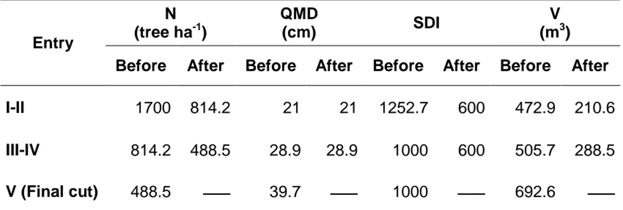
Table 6: Silvicultural management alternative showed in Figure 6. N: density (trees ha-1), QMD: quadratic mean diameter (cm), SDI: Reineke’s stand density index,V: the over bark volume (m3 ha-1).

Entry

N (tree ha-1)

QMD

(cm) SDI

V (m3)

Before After Before After Before After Before After

I-II 1700 814.2 21 21 1252.7 600 472.9 210.6

III-IV 814.2 488.5 28.9 28.9 1000 600 505.7 288.5

V (Final cut) 488.5 ــــــــ 39.7 ــــــــ 1000 ــــــــ 692.6 ــــــــ

Figure 6: Silvicultural management alternative for mixed stands of Pinus sylvestris and Pinus pinaster in the

Sierra de la Demanda

I II

II

I

IV

An example of a management alternative in this type of forest is showed in Table 6 and Figure 6. In this case a set of systematic thinning interventions were applied in two times and different intensities (I-II and II-III) and a final cut. The initial density was 1700 trees ha-1 and a quadratic mean diameter of 21 cm. The first systematic thinning was applied to obtain a density of 814.2 tree ha-1. Then the stand grew considering no natural mortality until a quadratic mean diameter of 28.9 cm, when the second systematic thinning should be applied. The density decrease from 814.2 trees ha-1 to 488.5 trees ha -1 _{after this second thinning. Again the stand grew until a quadratic mean diameter of}

approximately 40 cm, when the final cut should be applied.

Mixed-species stands as diverse systems: show a greater increment in above-ground woody biomass than pure-species stands (Vilà et al. 2007 ; Paquette and Messier 2011), for example, the annual woody biomass production of mixed stands in the Alto Tajo region in Spain, which consist of two pine species (Pinus sylvestris and Pinus nigra) and two oak species (Quercus ilex and Quercus faginea), exceed the production of monocultures stands by more than 48% (Jucker et al., 2014). Moreover, mixed stands have a higher level of carbon storage in root system (Brassard et al., 2011), in addition to their role in enriching wildlife taxa (Castagneyrol and Jactel 2012),

Our results showed that introducing a new variable reflects species mixing effects into the system of equations was not significant, while it was significant in other studies and was retained in the models to formulate SDMD (Swift et al., 2007; Tesfaye et al., 2016), indicating that there was no impact of species mixing on stand yield represented by quadratic mean diameter and over bark volume. That is contrary to what Riofrío et al (2018) concluded that at stand level for the two species in mixture stands, there was a shared gain in productivity with respect to varying tree growth responses to inter-specific competition for each species. In another study of mixed stands, but this time the mixture is a combination between Pinus sylvestris and Fagus sylvatica species, the results were similar to the previous one, where it showed increased productivity in the stands with superior growth of Pinus sylvestris than Fagus sylvatica growth which was reduced (Pretzsch et al., 2015).

Meaning that the behavior of our two species in mixed stands could be quite similar in term of productivity. Based on that, we led to only fit the system of models that uses stand density and dominant height, and quadratic mean diameter as independent endogenous variables.

These result should not be generalized about various site conditions because of differing productivity relationships on-site. Moreover there is a lack of knowledge for mixed stands although it is increasing during the last years: Pretzsch and Schütze, 2016; Riofrío et al., 2019... Different cases of site–growth relationships in mixed stands can be observed based on different site conditions: In the first case, when the interactions between the two species are absent, the stand mutual gain in productivity would result in a proportional increase of each species, it means the total productivity summarize the productivity of each species individually as in pure stands. In other cases, when there are interactions between both species, the total productivity is not the same than the sum of the individual productivities in pure stands, facilitative or competitive effects affect final productivity (Pretzsch, 2009b). In the present work the interaction between both species is not clear because mixture degree was not significant in the quadratic mean diameter and volume models.

inventory, plots consist of four circular subplots and minimum measured diameter at breast height is increasing along with subplots. Therefore expansion factors are necessary to know how many trees are representing each tree of NFI plots at hectare level. The number of trees to estimate the Assmann dominant height varies for each plot which complicates its estimation.

6. - CONCLUSIONS

- In the present master thesis a stand density management diagram for Pinus sylvestris and Pinus pinaster mixed forests from Sierra de la Demanda (Spain) has been developed. This diagram could be an easy tool for owners and managers of this region to manage mixed stands using simple variables like dominant height or density.

7.- ACKNOWLEDGMENTS

I would like to thank my mentors and thesis advisers, Felipe Bravo and Irene Ruano, for their support, encouragement, and most valuable advice. Their insight and feedback were essential in the process of completing this work. I would also like to express my profound gratitude to all the professors and people whom I consulted in writing this thesis and for imparting their knowledge over the course of my stay in this program, in particular, Lucía Risio Allione and Cristobal Ordóñez Alonso.

I would like to acknowledge José Antonio Bonet, the coordinator of the program in the University of Lleida for his personal support and mentorship. To José Borges, Erasmus Mundus Program Coordinator for the MEDFOR program, thank you for your patience, understanding, and having me in the program. For her delicate handling of our various concerns, I would like to thank Catarina Tavares, Erasmus Mundus Co-coordinator and Secretariat of MEDFOR.

I would like to thank the institutions which have been my home these past couple of years: the Escuela Técnica Superior de Ingeniería Agraria of the University of Lleida, Instituto Superior de Agronomia of the University of Lisbon, and Escuela Técnica Superior de Ingenierías Agrarias de Palencia of the University of Valladolid. Also, the Erasmus+ program and the MEDFOR consortium for accepting me and honing my abilities in this field.

8-. REFERENCES

Agalsa. (2006). Plan de Desarrollo Local 2007 – 2013. Junta de Castilla y León.

Alberdi, I., Cañellas, I., & Bombín, R. V. (2017). The Spanish National Forest Inventory: history, development, challenges and perspectives. Brazilian Journal of Forest Research/Pesquisa Florestal Brasileira, 37(91).

Ammer, C. (2016). Unraveling the importance of inter-and intraspecific competition for the adaptation of forests to climate change. In Progress in Botany Vol. 78 (pp. 345-367). Springer, Cham.

Anhold, J. A., Jenkins, M. J., & Long, J. N. (1996). Technical Commentary: Management of Lodgepole Pine Stand Density to Reduce Susceptibility to Mountain Pine Beetle Attack. Western Journal of Applied Forestry, 11(2), 50-53.

Assmann, E. (1970). The principles of forest yield study: studies in the organic production, structure, increment and yield of forest stands. Pergamon press.

Barrio Anta, M., & Álvarez González, J. G. (2005). Development of a stand density management diagram for even-aged pedunculate oak stands and its use in designing thinning schedules. Forestry, 78(3), 209-216.

Bengoa 1999. Estimación de la altura dominante de la masa a partir de la altura dominante de parcela. Ventajas frente a la altura dominante de Assman. Invest. Agr.: Sist. Recur. For.: Fuera de Serie n° 1.

Bengoa Martínez de Manjodana, J. (1999). Estimación de la altura dominante de la masa partir de la “altura dominante de parcela”. Ventajas frente a la altura dominante de Assman. Forest Systems, 8(3), 311-321.

Brassard, B. W., Chen, H. Y., Bergeron, Y., & Paré, D. (2011). Differences in fine root productivity between mixed‐and single‐species stands. Functional Ecology, 25(1), 238-246.

Burkhart, H. E. (2013). Comparison of maximum size–density relationships based on alternate stand attributes for predicting tree numbers and stand growth. Forest ecology and management, 289, 404-408.

Cabrera-Pérez, R. S., Corral-Rivas, S., Quiñonez-Barraza, G., Nájera-Luna, J. A., Cruz-Cobos, F., & Calderón-Leal, V. H. (2019). Density management diagram for mixed-species forests in the El Salto region, Durango, Mexico Diagrama de manejo de la densidad para los bosques mezclados de la región de El Salto, Durango. Revista Chapingo Serie Ciencias Forestales y del Ambiente, 25(1).

Cañellas, I., García, F. M., & Montero, G. (2000). Silviculture and dynamics of Pinus sylvestris L. stands in Spain. Forest Systems, 9(S1), 233-253.

Castagneyrol, B., & Jactel, H. (2012). Unraveling plant–animal diversity relationships: a meta‐regression analysis. Ecology, 93(9), 2115-2124.

Coll, L., Ameztegui, A., Collet, C., Löf, M., Mason, B., Pach, M., Verheyen, K., Abrudan, I., Barbati, A., Barreiro, S., Bielak, K., Bravo-Oviedo, A., Ferrari, B., Govedar, Z., Kulhavy, J., Lazdina, D., Metslaid, M., Mohren, F., Pereira, M., Peric, S., Rasztovits, E., Short, I., Spathelf, P., Sterba, H., Stojanovic, D., Valsta, L., Zlatanov, T., & Ponette, Q. (2018). Knowledge gaps about mixed forests: What do European forest managers want to know and what answers can science provide?. Forest Ecology and Management, 407, 106-115.

Dean, T. J., & Baldwin, V. C. (1993). Using a density-management diagram to develop thinning schedules for loblolly pine plantations. Res. Pap. SO-275. New Orleans, LA: US Department of Agriculture, Forest Service, Southern Forest Experiment Station. 12 p., 275.

Dean, T. J., & Baldwin, V. C. (1996). Crown management and stand density. In In: Carter, Mason C., ed. Growing trees in a greener world: industrial forestry in the 21st century; 35th LSU forestry symposium. Baton Rouge, LA: Louisiana State University Agricultural Center, Louisiana Agricultural Experiment Station: 148-159a-e..

Del Río, M., Pretzsch, H., Ruíz‐Peinado, R., Ampoorter, E., Annighöfer, P., Barbeito, I., I., Bielak, K., Brazaitis, G., Coll, L., Drössler, L., Fabrika, M., Forrester, D.I., Heym, M., Hurt, V., Kurylyak, V., Löf, M., Lombardi, F., Madrickiene, E., Matović, B., Mohren, F., Motta, R., den Ouden, J., Pach, M., Ponette, Q., Schütze, G., Skrzyszewski, J., Sramek, V., Sterba, H., Stojanović, D., Svoboda, M., Zlatanov, T.M., & Bravo-Oviedo, A. (2017). Species interactions increase the temporal stability of community productivity in Pinus sylvestris–Fagus sylvatica mixtures across Europe. Journal of Ecology, 105(4), 1032-1043.

Drew, T. J., & Flewelling, J. W. (1979). Stand density management: an alternative approach and its application to Douglas-fir plantations. Forest Science, 25(3), 518-532.

EUFORGEN. (2011). Pinus pinaster. Euforgen, 185(2–3), 1177–1186. https://doi.org/10.1016/j.jhazmat.2010.10.029

FOREST EUROPE, 2015. State of Europe’s Forests 2015. Status and trends in sustainable forest management in Europe.

Gamfeldt, L., Snäll, T., Bagchi, R., Jonsson, M., Gustafsson, L., Kjellander, P., Ruiz-Jaen, M.C., Froberg, M., Stendahl, J., Philipson, C.D., Mikusinski, G., Andersson, E., Westerlund, B., Andren, H., Moberg, F., Moen, J., & Bengtsson, J. (2013). Higher levels of multiple ecosystem services are found in forests with more tree species. Nature communications, 4, 1340.

Jack, S. B., & Long, J. N. (1996). Linkages between silviculture and ecology: an analysis of density management diagrams. Forest Ecology and Management, 86(1-3), 205-220.

Jactel, H., Bauhus, J., Boberg, J., Bonal, D., Castagneyrol, B., Gardiner, B., B., Gonzalez- Olabarria, J.R., Koricheva, J., Meurisse, N., & Brockerhoff, E.G. (2017). Tree diversity drives forest stand resistance to natural disturbances. Current Forestry Reports, 3(3), 223-243.

JCYL (Junta de Castilla y León), 2003. Plan Forestal de Castilla y León, tomo V3. Conservación y mejora de los bosques. Consejería de Medio Ambiente. 200 pp.

diversity–productivity relationships in Iberian forests. Journal of Ecology, 102(5), 1202-1213.

Kimsey Jr, M. J., Shaw, T. M., & Coleman, M. D. (2019). Site sensitive maximum stand density index models for mixed conifer stands across the Inland Northwest, USA. Forest Ecology and Management, 433, 396-404.

Kuehne, C., Kublin, E., Pyttel, P., & Bauhus, J. (2013). Growth and form of Quercus robur and Fraxinus excelsior respond distinctly different to initial growing space: results from 24-year-old Nelder experiments. Journal of Forestry Research, 24(1), 1– 14. https://doi.org/10.1007/s11676-013-0320-6

Lara, W., Bravo F., & Ordonez, C. (2018). Package ‘basifoR’ (not published yet)

Long, J. N. (1985). A practical approach to density management. The Forestry Chronicle, 61(1), 23-27.

Long, J. N., & Shaw, J. D. (2005). A density management diagram for even-aged ponderosa pine stands. Western Journal of Applied Forestry, 20(4), 205-215.

Long, J. N., Dean, T. J., & Roberts, S. D. (2004). Linkages between silviculture and ecology: examination of several important conceptual models. Forest ecology and management, 200(1-3), 249-261.

López-Sánchez, C., & Rodríguez-Soalleiro, R. (2009). A density management diagram including stand stability and crown fire risk for Pseudotsuga menziesii (Mirb.) Franco in Spain. Mountain Research and Development, 29(2), 169-177.

Marangon, G. P., Schneider, P. R., Zimmermann, A. P. L., Longhi, R. V., & Cavalli, J. P. (2017). DENSITY MANAGEMENT DIAGRAMS FOR STANDS OF Eucalyptus grandis W. Hill RS, BRAZIL. Revista Árvore, 41(1).

Mátyás, C., Ackzell, L., & Samuel, C. J. A. (2004). EUFORGEN technical guidelines for genetic conservation and use for Scots pine (Pinus sylvestris). Bioversity International. Montero, G., & Serrada, R. (2013). La situación de los bosques y el sector forestal en España: Informe ejecutivo: ISFE 2013. SECF.

Newton, P. F. (1997). Stand density management diagrams: Review of their development and utility in stand-level management planning. Forest Ecology and Management, 98(3), 251-265.

Newton, P. F., Lei, Y., & Zhang, S. Y. (2005). Stand-level diameter distribution yield model for black spruce plantations. Forest Ecology and Management, 209(3), 181-192.

Paquette, A., & Messier, C. (2011). The effect of biodiversity on tree productivity: from temperate to boreal forests. Global Ecology and Biogeography, 20(1), 170-180.

Patrício, M. D. S., & Nunes, L. (2017). Density management diagrams for sweet chestnut high-forest stands in Portugal. IForest, 10(6), 865–870.

Pretzsch, H. (2009a). Forest dynamics, growth, and yield. In Forest dynamics, growth and yield (pp. 1-39). Springer, Berlin, Heidelberg.

Pretzsch, H. (2009b). Effects of species mixture on tree and stand growth. In Forest Dynamics, Growth and Yield (pp. 337-380). Springer, Berlin, Heidelberg.

Pretzsch, H., & Schütze, G. (2016). Effect of tree species mixing on the size structure, density, and yield of forest stands. European journal of forest research, 135(1), 1-22.

Pretzsch, H., Del Río, M., Ammer, C., Avdagic, A., Barbeito, I., Bielak, K., ... & Fabrika, M. (2015). Growth and yield of mixed versus pure stands of Scots pine (Pinus sylvestris L.) and European beech (Fagus sylvatica L.) analysed along a productivity gradient through Europe. European Journal of Forest Research, 134(5), 927-947.

Puettmann, K. J., Wilson, S. M., Baker, S. C., Donoso, P. J., Drössler, L., Amente, G., Harvey, B.D., Knoke, T., Lu, Y., Nocentini, S., Putz, F.E., Yoshida, T., & Bauhus, J. (2015). Silvicultural alternatives to conventional even-aged forest management-what limits global adoption?. Forest Ecosystems, 2(1), 8.

Quiñonez-Barraza, G., Tamarit-Urias, J. C., Martínez-Salvador, M., García-Cuevas, X., Héctor, M., & Santiago-García, W. (2018). Maximum density and density management diagram for mixed-species forests in Durango, Mexico Densidad máxima y diagrama de manejo de la densidad para bosques mezclados de Durango, México. Revista Chapingo Serie Ciencias Forestales y del Ambiente, 24(1).

Reineke, L. H. (1933). Perfecting a stand-density index for even-aged forests. Journal of Agricultural Research, 46(7), 627–638.

Riofrío, J.(2018). Mixed stands growth dynamics of Scots pine and Maritime pine: species complementarity relationships and growth effects. Doctoral thesis. University of Valladolid, Spain.

Riofrío, J., del Río, M., & Bravo, F. (2016). Mixing effects on growth efficiency in mixed pine forests. Forestry: An International Journal of Forest Research, 90(3), 381-392.

Riofrío, J., del Río, M., Maguire, D. A., & Bravo, F. (2019). Species Mixing Effects on Height–Diameter and Basal Area Increment Models for Scots Pine and Maritime Pine. Forests, 10(3), 249.

Rivas-Martínez S, Rivas-Sáenz S (1996–2009) Sistema de Clasificación Bioclimática Mundial. Centro de Investigaciones Fitosociológicas, Spain. http://www.ucm.es/info/cif. Accessed 26 May 2011

Rodríguez, R. J., Serrada, R., Lucas, J. A., Alejano, R., Del Río, M., Torres, E., & Cantero, A. (2008). Selvicultura de Pinus pinaster Ait. subsp. mesogeensis Fieschi & Gaussen. In: Compendio de selvicultura aplicada en España. Edited by: Serrada, R., Montero, G., Reque, J. Instituto Nacional de Investigación y Tecnología Agraria y Alimentaria. Ministerio de Educación y Ciencia, Madrid, 399-430.

Schnell, S., Kleinn, C., & González, J. G. A. (2012). Stand density management diagrams for three exotic tree species in smallholder plantations in Vietnam. Small-scale Forestry, 11(4), 509-528.

Serrada, R., Montero, G., & Reque, J. A. (2008). Compendio de selvicultura aplicada en España (No. 634.95 C737). Instituto Nacional de Investigación y Tecnología Agraria y Alimentaria, Madrid (España) Ministerio de Educación y Ciencia, Madrid (España).

Sharma, M., & Zhang, S. Y. (2007). Stand density management diagram for jack pine stands in eastern Canada. Northern Journal of Applied Forestry, 24(1), 22-29.

Shaw, J. D., & Long, J. N. (2007). A density management diagram for longleaf pine stands with application to red-cockaded woodpecker habitat. Southern Journal of Applied Forestry, 31(1), 28-38.

Swift, E., Penner, M., Gagnon, R., & Knox, J. (2007). A stand density management diagram for spruce–balsam fir mixtures in New Brunswick. The forestry chronicle, 83(2), 187-197.

Tang, X., Pérez-Cruzado, C., Vor, T., Fehrmann, L., Álvarez-González, J. G., & Kleinn, C. (2015). Development of stand density management diagrams for Chinese fir plantations. Forestry: An International Journal of Forest Research, 89(1), 36-45.

Tesfaye, M. A., Bravo, F., & Bravo-Oviedo, A. (2016). Alternative silvicultural stand density management options for Chilimo dry afro-montane mixed natural uneven-aged forest using species proportion in Central Highlands, Ethiopia. European journal of forest research, 135(5), 827-838.

Vacchiano, G., Derose, R. J., Shaw, J. D., Svoboda, M., & Motta, R. (2013). A density management diagram for Norway spruce in the temperate European montane region. European journal of forest research, 132(3), 535-549.

Valbuena, P., Del Peso, C., & Bravo, F. (2008). Stand density Management Diagrams for two Mediterranean pine species in Eastern Spain. Forest Systems, 17(2), 97-104.

Van Der Plas, F., Manning, P., Allan, E., Scherer-Lorenzen, M., Verheyen, K., Wirth, C., Zavala, M.A., Hector, A., Ampoorter, E., Baeten, L., Barbaro, L., Bauhus, J., Benavides, R., Benneter, A., Berthold, F., Bonal, D., Bouriaud, O., Bruelheide, H., Bussotti, F., Carnol, M., Castagneyrol, B., Charbonnier, Y., Coomes, D.A., Coppi, A., Bastias, C.C., Muhie Dawud, S., De Wandeler, H., Domisch, T., Finér, L., Gessler, A., Granier, A., Grossiord, C., Guyot, V., Hättenschwiler, S., Jactel, H., Jaroszewicz, B., Joly, F.X., Jucker, T., Koricheva, J., Milligan, H., Müller, S., Muys, B., Nguyen, D., Pollastrini, M., Raulund-Rasmussen, K., Selvi, F., Stenlid, J., Valladares, F., Vesterdal, L., Zielínski, D., & Fischer, M. (2016). Jack-of-all-trades effects drive biodiversity–ecosystem multifunctionality relationships in European forests. Nature communications, 7, 11109.

Vanclay, J. K., Lamb, D., Erskine, P. D., & Cameron, D. M. (2013). Spatially explicit competition in a mixed planting of Araucaria cunninghamii and Flindersia brayleyana. Annals of Forest Science, 70(6), 611–619. https://doi.org/10.1007/s13595-013-0304-x

VanderSchaaf, C. L., & Burkhart, H. E. (2012). Development of Planting Density– Specific Density Management Diagrams for Loblolly Pine. Southern Journal of Applied Forestry, 36(3), 126-129.

ANNEX 1 STATSTICAL SCRIPT

####################################################################### #### SDMD for mixed stands of Pinus sylvestris and Pinus pinaster ##### ####################### in Demandas mountains ######################### #######################################################################

### work directory ###

setwd('E:/MScThesis_MEDFOR_UVa/Data/Processed')

################################################ ################ Data selection ################ ################################################

### Packages and libraries:

install.packages("Hmisc")

install.packages(pkgs='E:/MScThesis_MEDFOR_UVa/Data/

Processed/Rbasifor/Rbasifor_0.1.tar.gz', repos = NULL)

library(measurements)

library(Hmisc)

library(RODBC)

# package to extrac and compute variables from Spanish National Forest Inventory:

library(Rbasifor)

# help(Rbasifor)

library(foreign)

## read tree data from url using Rbasifor:

bu.tree <- readNFI('https://www.mapama.gob.es/es/biodiversidad/

servicios/banco-datos-naturaleza/ifn3p09_tcm30-29392

3.zip')

so.tree <- readNFI('https://www.mapama.gob.es/es/biodiversidad/

servicios/banco-datos-naturaleza/ifn3p42_tcm30-29398

9.zip')

####################################################################### ######################### volume calculation ########################## #######################################################################

### First calculate dendrometric variables to use metics2Vol function:

## Burgos provinces:

bu.de.met <- nfiMetrics(bu.tree) #(Burgos_dendrometric variables)

burgos <- metrics2Vol(bu.de.met)

head(burgos)

# Dendrometrics at plot level:

burgos.p <- dendroMetrics(burgos)

####################################################################### ### A new coefficient represent the proportions of the species in ##### ### the mixed stands (Pinus sylvestris as a reference)(Burgos): ####### #######################################################################

## P.sylvestris basal area (tree level)(m^2/tree)

bu.bas.P.syl<- burgos[burgos$Especie=="21",]

# P.sylvestris basal area per ha (tree level)(m^2/ha)

bu.bas.P.syl <- dendroMetrics(bu.bas.P.syl)

names(bu.bas.P.syl)[names(bu.bas.P.syl) == "ba"] <- "p.syl_ba"

bu.bas.P.syl$prv_plot <- with(bu.bas.P.syl, paste(pr, Estadillo, sep='

_'))

head(bu.bas.P.syl)

####################################################################### ## Soria provinces:

so.de.met<- nfiMetrics(so.tree) #(Soria_dendrometric variables)

soria <- metrics2Vol(so.de.met)

head(soria)

# Dendrometrics at plot level:

soria.p <- dendroMetrics(soria)

head(soria.p)

####################################################################### ### A new coefficient represent the proportions of the species in ##### ### the mixed stand (Pinus sylvestris as a reference)(Soria): ######### #######################################################################

## P.sylvestris basal area (tree level)(m^2/tree)

so.bas.P.syl<- soria[soria$Especie=="21",]

# P.sylvestris basal area per ha (tree level)(m^2/ha)

so.bas.P.syl <- dendroMetrics(so.bas.P.syl)

names(so.bas.P.syl)[names(so.bas.P.syl) == "ba"] <- "p.syl_ba"

so.bas.P.syl$prv_plot <- with(so.bas.P.syl, paste(pr, Estadillo, sep='

_'))

head(so.bas.P.syl)

########################################################### ###### Dominant height calculation ######################## ###########################################################

### Burgos:

bu.test<- nfiMetrics(bu.tree) #(Burgos_dendrometric variables)

head(bu.test)

bu.syl<- bu.test[bu.test$Especie==21,]

bu.pin<- bu.test[bu.test$Especie==26,]

bu.pinus <- rbind (bu.syl,bu.pin)

head(bu.pinus)

bu.pinus$d <-(bu.pinus$d/10)

bu.pinus$h<-(bu.pinus$h/10)

max(bu.pinus$Especie)

## loop to calculate the dominante height (Burgos) :

plots<-bu.pinus$Estadillo

bu.domH<-data.frame()

for (i in plots){

# i<-45

# Plots selection:

plot.i<-bu.pinus[bu.pinus$Estadillo==i,]

# if (plot.i$Estadillo>0)

# Order plot i according to DBH (bigger to smaller)

ordering<-plot.i[order(plot.i$d,decreasing=TRUE),]

# Calculate cumulative sums of the expansion factor:

ordering$sum.exp.fact <- cumsum(ordering$n)

# Select rows until 100 of cumulative sum of expansion factor:

select.Pi <- ordering[0:(nrow(ordering[ordering$sum.exp.fact<100,]))+

1,]

if (nrow(select.Pi)>1) {

## we are going to change expansion factor of the last tree to # obtain exactly 100 trees per hectare:

new.exp.fact <- replace(select.Pi$n,select.Pi$sum.exp.fact>=100,100

-select.Pi

[nrow(select.Pi)-1,'sum.exp.fact'])

select.Pi<-as.data.frame(select.Pi) # select.Pi is a list, not a da

taframe

select.Pi <-cbind(select.Pi,new.exp.fact)

select.Pi$sum.exp.fact2 <- cumsum(select.Pi$new.exp.fact)

# dominant height

Ho<-sum(select.Pi$h*select.Pi$new.exp.fact)/100

}else{

if (select.Pi$n>100){

Ho<- select.Pi$h

}else{

Ho<- 0

Estadillo <-i

domH<-cbind(Estadillo,Ho)

bu.domH<-rbind(bu.domH,domH)

}

bu.domH <- na.omit(bu.domH)

bu.domH<-unique(bu.domH)

max(bu.domH$Ho)

bu.domH$prv_plot <- with(bu.domH, paste("9", Estadillo, sep='_'))

head(bu.domH)

write.csv(bu.domH,file="bu.domH.csv")

############################################################### ###############################################################

### Soria:

so.test<- nfiMetrics(so.tree) #(Soria_dendrometric variables)

head(so.test)

so.syl<- so.test[so.test$Especie==21,]

so.pin<- so.test[so.test$Especie==26,]

so.pinus <- rbind (so.syl,so.pin)

so.pinus <- na.omit(so.pinus)

head(so.pinus)

so.pinus$d <-(so.pinus$d/10)

so.pinus$h<-(so.pinus$h/10)

max(so.pinus$Especie)

###loop to calculate the dominante height (Soria) :

plots<-so.pinus$Estadillo

so.domH<-data.frame()

for (i in plots){

# i<-45

# Plots selection:

plot.i<-so.pinus[so.pinus$Estadillo==i,]

# if (plot.i$Estadillo>0)

# Order plot i according to DBH (bigger to smaller)

ordering<-plot.i[order(plot.i$d,decreasing=TRUE),]

# Calculate cumulative sums of the expansion factor:

ordering$sum.exp.fact <- cumsum(ordering$n)

# Select rows until 100 of cumulative sum of expansion factor:

select.Pi <- ordering[0:(nrow(ordering[ordering$sum.exp.fact<100,]))+

1,]

if (nrow(select.Pi)>1) {

## we are going to change expansion factor of the last tree to # obtain exactly 100 trees per hectare:

new.exp.fact <- replace(select.Pi$n,select.Pi$sum.exp.fact>=100,100

-select.Pi

[nrow(select.Pi)-1,'sum.exp.fact'])

select.Pi<-as.data.frame(select.Pi) # select.Pi is a list, not a da

taframe

select.Pi <-cbind(select.Pi,new.exp.fact)

select.Pi$sum.exp.fact2 <- cumsum(select.Pi$new.exp.fact)

# dominant height

Ho<-sum(select.Pi$h*select.Pi$new.exp.fact)/100

}else{

if (select.Pi$n>100){

Ho<- select.Pi$h

}else{

Ho<- 0

} }

Estadillo <-i

domH<-cbind(Estadillo,Ho)

so.domH<-rbind(so.domH,domH)

}

so.domH <- na.omit(so.domH)

so.domH<-unique(so.domH)

max(so.domH$Ho)

so.domH$prv_plot <- with(so.domH, paste("42", Estadillo, sep='_'))

head(so.domH)

write.csv(so.domH,file="so.domH.csv")

################################################# ## join data frames of "bu.domH" and "so.domH":## #################################################

bu.so.domH <- rbind (bu.domH,so.domH)

############################################################ ###### selecting mixed plots in Demandas mountains ######### ############################################################

## Makeing a new variable joins "Provincia" and "Estadillo" # in both data frames of Bugros and Soria (estadillo is plot:

head(burgos.p)

soria.p$prv_plot <- with(soria.p, paste(pr, Estadillo, sep='_'))

head(soria.p)

## join data frames of "burgos.p" and "soria.p":

bu.so.p <- rbind (burgos.p,soria.p)

head(bu.so.p)

## join data frames of "bu.bas.P.syl" and "so.bas.P.syl":

bu.so.bas.P.syl <- rbind (bu.bas.P.syl,so.bas.P.syl)

head(bu.so.bas.P.syl)

### selecting the mixed plots in Demandas mountains: ####################################################

library("foreign", lib.loc="C:/Program Files/R/R-3.4.0/library")

demanda <- read.dbf("IFN-PsPt-Demanda.dbf")

head(demanda)

## Makeing a new variable joins "Provincia" and "Estadillo" # in the data frame of Demandas mountains:

demanda$prv_plot <- with(demanda, paste(Provincia, Estadillo, sep='_')

)

head(demanda)

## selecting the mixed plots:

demanda.mix <- demanda[demanda$Type=="M",]

head(demanda.mix)

####################################################################### # selecting the common mixed plots between "demanda.mix" and "bu.so.p":

data.de <- bu.so.p[which(bu.so.p$prv_plot %in% demanda.mix$prv_plot),]

head (data.de)

# Merging and selecting common mixed plots between "data.de" and "bu.so .bas.P.syl"

data.de.2<- merge(data.de,bu.so.bas.P.syl ,by="prv_plot")

head(data.de.2)

data.de.3<-data.de.2[,c("prv_plot","pr.x","Especie.x","X.x","Estadillo.

x","ba",

"p.syl_ba","d.x","dg.x","h.x","n.x","v.x")]

head(data.de.3)

names(data.de.3)[names(data.de.3) == "pr.x"] <- "pr"

names(data.de.3)[names(data.de.3) == "Especie.x"] <- "Especie"

names(data.de.3)[names(data.de.3) == "X.x"] <- "X"

names(data.de.3)[names(data.de.3) == "Estadillo.x"] <- "Estadillo"

names(data.de.3)[names(data.de.3) == "d.x"] <- "d"

names(data.de.3)[names(data.de.3) == "dg.x"] <- "dg"

names(data.de.3)[names(data.de.3) == "h.x"] <- "h"

names(data.de.3)[names(data.de.3) == "n.x"] <- "n"