Addressing Endogeneity in the Relationship Between Health
and Employment Through a Simultaneous Equations Model
Empirical Study for USA
Daniel Andr´es Pinz´on Fonseca MSc. in Economics
Colegio Mayor Nuestra Se˜nora del Rosario Master Thesis
Bogot´a, Colombia
August 2012
Abstract
This document examines the two-way relationship between health and employ-ment and their dynamics using U.S. data from the PSID (Panel study of Income Dynamics). This study uses two dependent variables (Self-assessed health and Em-ployment) which are estimated using a bivariate probit model to address the endo-geneity problem present between them. The results show that there is a significant evidence of the existence of endogeneity and suggest that good health positively affects the probability of being employed (healthy people have 2.85% more chances to join the labour force than unhealthy people) and that there is a positive im-pact of being employed on the probability of reporting good health (employees have 0,07% more chances of being healthy than non-employees), however, the effect of employment status on health is found not significant.
1
Introduction
Ageing population and its sustainability has been an international concern in the last decades. The United Nations Economic Commission for Europe have this issue as one of its main topics, showing the importance that it is getting nowadays. This is a worlwide discussion which have made some governments to contemplate the possibility of incre-menting the retirement age. This decision could amplify the labour market, however, health is needed to make this extra force efficient and hold or improve the productivity of the economy.
The literature have shown that the effect of health on employment is positive, (e.g. Dooley et al. [1996], Clark and Oswald [1994], Bambra and Eikemo [2009], Morris et al. [1994]). Healthy people are more likely to be employed than those who report to be unhealthy Pelkowski and Berger [2004]). Garc´ıa-G´omez et al. [2010] showed that health limitations increase the hazard of non-employment by 58% for men and by 39% for women. Further-more, the decision to join or leave the labour market strongly depends on the individual’s health status, because unhealthy people may decide to be unemployed or continue in their non-employment status due to their health, or they can lose their job because of their low productivity.
It is also known that the effect of employment on health (e.g. B¨ockerman and Ilmakunnas [2007], Dooley et al. [1996], Clark and Oswald [1994], Bambra and Eikemo [2009], Mor-ris et al. [1994]) is also positive. Employed people usually report a better health status than those who are unemployed (in some studies authors use non-employed instead of unemployed), for instance, Rodriguez [2002] shows that full-time employed people with fixed-term contracts in Germany are about 42% more likely to report poor health than those who have permanent work contracts. Moreover, the lack of employment may impact individual’s mental health and this can be reflected later in physical health problems (Jin et al. [1997]).
Endogeneity problems are important issues that have to be considered in order to explain the relationship between health and employment. Most of the articles in the literature have addressed this problem by instrumental variables and others by simultaneous equa-tions.
Following Haan and Myck [2009], who analyzed this relationship and their dynamics us-ing a bivariate probit model and panel data for Germany, the aim of this document is to analyze the double causality found in health and employment and their dynamics pro-viding evidence for The USA (United States) using the PSID (Panel Study of Income Dynamics) from 1985 to 2007 (18 waves). The results obtained in this study are congru-ent to the literature showing the positive relationship between health and employmcongru-ent. Furthermore, the results show that a healthy person has a higher chance to be employed than an unhealthy person (an increase of 2,85% of the probability of being employed); they also show that an employed individual has an increase of 0,07% of the probability of reporting a good health status compared to a non-employed individual, however, the effect of employment on health is found to be not significant.
2
Literature Review
sev-eral and major problems on the health status. People who are not employed are tending to generate cardiovascular, physical, medical and mental disorders. Furensgaard et al. [1983] tested the psychosocial characteristics of a group of unemployed patients consec-utively admitted to a psychiatric emergency department, and found that persons who are under anxiety can also develop many other problems causing suicidal desires, alcohol consumption and physiological illness.
The association of unemployment and health has also been studied using morbidity and mortality as a measure of health (Bambra and Eikemo [2009], Morris et al. [1994]). Bam-bra and Eikemo [2009] used the European Social Survey from 2002 to 2004 within the population between 25 and 65 years-old for 23 countries (Scandinavian, Anglo-Saxon, Bismarckian, Southern and Eastern), to test the relationship between unemployment and self-reported health using risk morbidity and mortality as a measure for the health sta-tus. They show that people who were unemployed had higher rates of mortality and poorer health than those who were employed. Additionally, health problems predomi-nately ocurred for women who are themselves are more likely to receive less than the average wage than men. Repetti et al. [1989] found this differential effect of gender on health, showing that employment among women is significantly related to better health (positive). Using a cohort study in Britain from 1978 to 1985 for middle-aged men, Morris et al. [1994] found that men who experienced unemployment were twice more likely to die than men who remained continuously employed.
Using probability models, Rodriguez [2002] examined the impact of marginal employment based on panel data from Britain and Germany (1991-1993), including both temporary and part-time employment schemes where the measure of the perceived health status is used as the dependant variable. They show that, fulltime employed people with fixed-term contracts in Germany are about 42% more likely to report poor health than those who have permanent work contracts. In Britain, only part-time work with no contract is associated with poor health, but the difference is not statistically significant.
In order to explain the causal effect between health and employment, it should be taken into account problems of endogeneity, this mean that the independent variable is corre-lated with the error term because the existance of ommited variables or simultaneity in dynamics models. In the literature, there are two main methods used to address endo-geneity problems: instrumental variables and simultaneous equations.
Some instrumental variables that have been used to tackle the endogeneity are: self re-ported measured of limitations in physical functioning (Zucchelli et al. [2010]), initial health and lagged health (Garc´ıa-G´omez et al. [2010]), early and full statutory retirement ages (Coe and Zamarro [2011]), public pension policies1
(Rohwedder and Willis [2010]), activities of daily living ADLs (Kalwij and Vermeulen [2008], Bound et al. [1999]), body mass Index BMI (Kalwij and Vermeulen [2008]), health shocks (Lindeboom et al. [2006]) and hospital diagnoses (Jakobsen and Larsen [2010]).
In a literature review of studies which tackle endogeneity by the use of instrumental
vari-1
ables, Currie and Madrian [1999] show empirical evidence of the effects of health on the labour market activity, as they showed that poor health is related to lower wages which is caused by various channels. In general, health impacts the labour market outcomes through its direct effect on productivity, and indirectly by altering trade-offs between income and leisure but there is no clear evidence for the magnitude of the estimated re-lationship.
Moreover, using data from the National Longitudinal Surveys (NLS) of Older Men in 1976 and Mature Women in 1977 (USA) it has been showed that current permanent health conditions have significant negative effects on the average hourly wages of workers (Pelkowski and Berger [2004]). Other studies used the the HRS (Health and Retirement Survey) to show that in the USA, the rate to enter the labour force is 7% lower for a man who reports a bad health status than for a man in fair health (Blau and Gilleskie [2001]) and that when a health shock occurs in early ages, it is less likely to lead to labour force exits (Bound et al. [1999]). Bound et al. [1999] found evidence that only 30% of men remained in the labour force whose health was good in the second wave of the HRS and then later declined. Likewise, Brown et al. [2005] showed that diabetes has negative impact on employment and labour productivity, indicating that the probability of em-ployment of diabetics is 7,4% to 7,5% lower than for non-diabetics.
In contrast to the USA, in Autralia using the HILDA (Houshold, Income and Labour Dy-namics in Australia) survey, it has been found that health shocks increase the propability of leaving the labour force by 50%, while in presence of limitations the propability even increases to 122% (Zucchelli et al. [2010]). Using wages as a proxy of the labour market, health has a positive and significant effect on wages, however,the effect of wages on health is found insignificant (Cai [2007]). The later result is found as well by Leung and Wong [2002] using a large cross-sectional data set, obtained from a survey of the Hong Kong population as they concluded that there is strong evidence that the health status is a significant determinant of employment, but not vice versa.
Analyzing the effect of retirement on cognition using cross-nationally comparable surveys of older people in The USA, England and 11 European countries for 2004. Rohwedder and Willis [2010] found that retirement is associated with a reduction of the memory score compared to those who continued working. The causal effect of retirement on health is identified by using a two-stage estimation method with public pension policies (number of years to or since reaching the age of eligibility for early retirement benefits and for full retirement benefits) as instrumental variables. Furthermore, in contrast to Rohwedder and Willis [2010], Coe and Zamarro [2011] using two steps estimations and early and full statutory retirement ages as instrumental variables, with data taken from the Survey of Health, Ageing and Retirement in Europe (SHARE), they conclude that retirement induced by social security leads to a 0.35 point decrease in the probability of reporting to be in fair, bad or very bad health. Additionally, using the SHARE it has been shown that a man who reports a good health status has higher chances to participate in the labour force, between 13,2% in Greece and 28,8% in Germany, than a man who reports bad health status (Kalwij and Vermeulen [2008]).
specific European countries. In Denmark, Jakobsen and Larsen [2010] examined the causal effect of health on employment and show that new diagnoses indicating poor health reduce the probability of employment in about 46% for immigrants and by about 39% for Danish natives. On the other hand, Lindeboom and Kerkhofs [2009] using the Leiden University Center for Research on Retirement and Ageing (CERRA) panel survey for 1993 and 1995 in The Netherlands, showed that financial incentives are important factors for the deci-sion to stop working (pendeci-sion reforms). Furthermore, they concluded that pendeci-sion and social security reforms made in order to increase labour participation of elderly may have adverse effects on their health because the increased working efforts for older ages result in a deterioration of health.
In Great Britain using data from the National Child Development Study, Lindeboom et al. [2006] showed that that when disability occurs at the age of 25, the employment rate at the age of 40 is reduced by 21%. Furthermore, they conluded that people who experienced bad health conditions during early childhood show a higher tendency to de-velop health deterioration during adulthood and to become non-employed than those who have not experienced bad conditions during childhood. Garc´ıa-G´omez et al. [2010] using the BHPS (British Household Panel Survey) found a positive relationship between health and employment, showing that presences of health limitations increase the propability of leaving the labour force by 58% for men and by 39% for women. Moreover, they show that mental health decay increases the risk of non-employment and also that mental health improvement does not increase the level of employment.
Although there is a scarce of this kind of studies using panel data, Haan and Myck [2009] proposed a joint model of health and labour market risks which identifies the mechanism through which poor health contributes to the probability of being jobless and vice versa. They used non-employment as the expression of labour market risk and Self-assessed health status (SAH) as a measure of health risk. Thus, they estimated a dynamic bivari-ate logit model in which they explained the joint distribution of unobserved heterogeneity in a non-parametric way. The analysis has been realized on the sample of German men aged 30-59 using the German Socio-Economic Panel (SOEP) data for the years 1996-2007 and the results confirm a strong and significant relationship between health and labour market risks. Authors found evidence for positive correlation in unobservable characteris-tics determining the two risks which indicates that a separate treatment would lead to an overestimation of the relationship and finally they found ceteris paribus a positive effect of poor health on the labour market risk.
In colcusion, as it can be seen from the literature there is a positive relationship between health and employment. Healthy people are more likely to be employed than those who are unhealthy because health limitations increase the hazard of non-employment and the decision to join or leave the labour market. On the other hand, employed people usu-ally report a better health status than those who are unemployed, additionaly, the lack of employment may impact individual’s mental health and this can be reflected later in physical health problems.
from the relationship, it allows as well to study the dynamics of health and employment; moreover, it allows controlling for individual unobserved heterogeneity (individual fixed effects) taking into account the whole range of working-age.
3
Methodology
The main objective of this study is to understand the dynamics of health and employment and their relationship taking advantage of a panel data. The model proposed in this study is a simultaneous equations bivariate probit model. Using a panel data from the PSID, I take into account the individual heterogeneity problem through fixed effects and use the method proposed by Wooldridge [2005] to correct the intial conditions problem.
The model proposed, which is setted up later on, have two dependant variables, health (SAH) and employmentand is based on the following expressions:
P(Hit = 1) =f(α1+β2Ht−2+β3Et−2+ Υ1Ξit+ Ω1Y ear+ Ψit) (1)
P(Eit= 1) =f(α2+γ2Ht−2+γ3Et−2+ Υ2Ξit+ Ω2Y ear+ Φit) (2)
The first equation specifies the relationship between Self-assessed Health (SAH) which is captured by the variable named health (H) and other explanatory variables includ-ing employment; the second equation specifies the relationship between employment and other explanatory variables including health (SAH).
In the equations above, i represents individuals and t represents years, H denotes the Self-Assessed Health (SAH - health status) and E denotes Employment, Ht−2 and Et−2
captures the SAH and the employment condition in the previous period respectively. One of the parameters that appear in the equations above is Ξ, which is a vector that contains the socio-economic and socio-demographic control variables (Age, Sex, Race, Income, Ed-ucation, number of household members, Own House, Health insurance, Marital Status, Disability and Race). The econonomical cycle is captured using dummy variables which are contained in the vector Y ear and the parameters Ψ and Φ are the error terms and
α1 and α2 are constant terms. Notice that, β2, β3, Υ1, Ω1 γ2, γ3, Υ2 and Ω2 are the
coefficients attached to the respective variables in each equation.
The individual heterogeneity problem is solved through an individual fixed effects set up, following the method proposed by Mundlak [1978]. Additionally, there is an initial conditions problem that arises for nonlinear panel data with unobservable heterogeneity (Heckman [1981]). This problem is that the initial observations (t = 0) are not random and correlated with the unobservable effects (Haan and Myck [2009]), such as how peo-ple value their health. The later problem is solved following the method proposed by Wooldridge [2005], who includes the initial condition of the dependent variable into the error term.
The following expressions show the corrections mentioned above:
ui = Λ2Ξi +γ2E0+δi; δi ∼N(0, σδ2) (4)
Thus, substituting equation (3) into Ψit = vi +ǫit and equation (4) into Φit = ui +ϕit leads to
Ψit = Λ1Ξi +β1H0+ϑi+ǫit (5)
and
Φit= Λ2Ξi+γ2E0+δi+ϕit, (6)
where Ξi is a vector which contains the mean of the variables included in Ξ over time of individuali.
Then, substituting equations (5) and (6) into (1) and (2) respectively, and, setting up a si-multaneous equations system with the resulting equations in order to address endogeneity, leads to:
P(Hit= 1) =f(α1+β2Ht−2+β3Et−2+ Υ1Ξit+ Ω1Y ear+ Λ1Ξi+β1H0+ϑi+ǫit) (7)
and
P(Eit = 1) =f(α2+γ2Ht−2+γ3Et−2+ Υ2Ξit+ Ω2Y ear+ Λ2Ξi+γ2E0+δi+ϕit) (8)
with
ϕit
ǫit
∼N(0,Σ) where: Σ =
1 σϕǫ
σǫϕ 1
.
Thus, holding the assumption of endogeneity (the error terms of eq.(7)ϕit are correlated with the error terms of eq.(8) ǫit) the bivariate probit model (simultaneous equations of two discrete dependent variables) proposed in this study to estimate the relationship between health and employment is given by equations (7) and (8). Notice that because of the scarce of instrumental variables, it is assumed that health and employment are affected by the last period’s conditions (Garc´ıa-G´omez et al. [2010]). This assumption allows to use the lag variables of health and employment into the equations to estimate this simultaneous system.
4
Data and Variables
4.1
Data
to 2007.
The Health chapter started in 1985 and it has been mostly focused on the households heads and their partners. Thus, this study only includes the aged-working population of this group (between 16 and 65 years-old).The final sample is 27.268 individuals (134.549 observations given that not all individual are obeserved every year).
4.2
Variables
4.2.1 Health: Self-assessed Health (SAH)
In order to analyze the individual’s health status, there is a question in the PSID’s ques-tionnaire where the individual is asked to value its own health at the time of the interview by choosing one of the following five options: Excellent (1), Very Good (2), Good (3), Fair (4) and Poor (5).
Because of the econometric specification, these five categories are recategorized into two categories. The first one collects the following categories: Excellent, Very Good and Good; and the second collects the remainig two options.
4.2.2 Employment
The employment status is collected by asking the individual about its current situation, offering eight options: (1) Working now, (2) Only temporarily laid off, sick leave or ma-ternity leave, (3)Looking for work, unemployed, (4) Retired, (5) Permanently disabled, temporarily disabled, (6) Keeping house, (7) Student and (8) Other.
These categories are reorganized into two categories. One of the new categories is Em-ployed which collects the categories (1) Working now and (2) Only temporarily laid off, sick leave or maternity leave ; and the other is non-employed which collects the other six categories.
4.2.3 Socio-Economic and Socio-Demographic variables
These kind of variables are used as control variables because they can influence the individ-ual’s health and employment status. The variables summerized as the Socio-Demographic variables are: Age, Sex, Marital Status (Single, Widowed, Divorced or Separated and the base category is Married), Race (White, Black and the base category is Other), Num-ber of household memNum-bers and Health Insurance. Variables’ names and description are represented in table 1.
Table 1: Variables included in the study
Variable Description
Age Age of the Individual (in years).
continued from previous page
Variable Description
the type or amount of work, 0 Otherwise. Education Years of Schooling.
Employment 1 If the Individual is employed, 0 Otherwise.
Health 1 If the Self Auto-reported Health Status is good or very good, 0 Otherwise.
Health Insurance 1 If the Individual is covered by an insurance, 0 Otherwise. log(Income) Logarithm of total household Income,
adjusted by the Consumer Index Price. # Members Fu Number of Household members.
Own House 1 If the individual lives in its own house, 0 Otherwise. Sex 1 If the individual is Male, 0 if Female.
MARITAL STATUS
Married 1 If the individual is Married, 0 Otherwise. (Reference Category) Single 1 If the individual is Single, 0 Otherwise.
Widowed 1 If the individual is Widowed, 0 Otherwise. Divorced 1 If the individual is Divorced, 0 Otherwise. Separated 1 If the individual is Separated, 0 Otherwise.
RACE .
White 1 if the race of the individual is White, 0 otherwise. Black 1 if the race of the individual is Black, 0 otherwise. Other 1 if the race of the individual is not White neither Black,
0 otherwise. (Reference Category)
[image:9.612.84.529.72.420.2]4.3
Descriptive statistics
Table 22
represents the descriptive statistics of the whole sample, the people employed/non-employed, the people with good/poor health, healthy employees and non-healthy unem-ployees. The average age of the individuals in the sample is 39.41 years and 45% of them are males. In this sample, 86% of the observations reported at least a good health status at the time of the interview and 76% reported to be employed.
Table 2: Descriptive Statistics
1985 - 2007(Odd Years)
All E=1 E=0 H=0 H=1 E=1 E=0
& H=1 & H=0
Mean Mean Mean Mean Mean Mean Mean
Health 0.86 0.91 0.71 0.00 1.00 1.00 0.00
Employment 0.76 1.00 0.00 0.48 0.80 1.00 0.00
Sex 0.45 0.51 0.26 0.40 0.46 0.51 0.33
Age 39.41 38.69 41.66 45.42 38.46 38.28 47.68
continued on next page
2
continued from previous page
1985 - 2007(Odd Years)
All E=1 E=0 H=0 H=1 E=1 E=0
& H=1 & H=0
Mean Mean Mean Mean Mean Mean Mean
# Members FU 3.13 3.11 3.20 3.09 3.13 3.10 3.02
Own 0.60 0.63 0.51 0.52 0.62 0.64 0.47
log(Income) 10.73 10.91 10.15 10.17 10.82 10.95 9.79
Health Insurance 0.40 0.40 0.40 0.40 0.40 0.40 0.43
Disability 0.14 0.08 0.32 0.53 0.08 0.06 0.72
Education 12.79 13.12 11.78 11.07 13.06 13.25 10.47
Married 0.68 0.69 0.62 0.57 0.69 0.70 0.54
Single 0.16 0.15 0.18 0.15 0.16 0.15 0.15
Widowed 0.02 0.02 0.04 0.06 0.02 0.01 0.09
Div/Sep 0.14 0.14 0.16 0.21 0.13 0.13 0.22
White 0.63 0.65 0.56 0.48 0.65 0.67 0.46
Black 0.29 0.27 0.34 0.42 0.27 0.26 0.43
Other Race 0.08 0.07 0.09 0.11 0.07 0.07 0.11
N 134,549 101,974 32,575 18,285 116,264 93,157 9,468
Source: PSID Data, waves 1985 - 2007 E=1: Employed; E=0: Non-employed H=1: Healthy; H=0: Unhealthy
From those individuals employed, 91% reported to be healthy, while this percentage de-creases to 71% for the group of non-employed individuals. On the other hand, 80% of the healthy individuals reported to be employed while this figure decreases to 48% for the unhealthy individuals.
The average age of the healthy-employed individuals is 38.28 years while it is 47.68 for the unhealthy-non-employed individuals. The education level is another difference between these groups because in the first group, the average duration of schooling is 13.25 years while in the second group it is 10.47 years. Finally, the main difference between healthy-employed and unhealthy-non-healthy-employed groups is given by disability, in this case, 6% of the healthy-employed individuals were disabled and this figure rises to 72% for the other group.
[image:10.612.88.522.75.354.2]The relationship between Health and employment could be obtained from transition ma-trices of health and employment which are shown inTable 3. The first row of the table shows the probability to change between estates of health conditioned by the employment status of the previous time period; and the second row of the table shows the transition of employment conditioned to the individual’s health status of the previous time period.
Table 3shows a positive relationship between health and employment status. This table shows that an individual who was employed at time (t−2) and reports a bad health status
Table 3: Health and Employment Transition Matrices. Sample:1985-2007 (Odd years)
Health t+ 2
Ht+2 = 0 Ht+2 = 1
Health t Ht = 0 53.50% 46.50%
Ht = 1 5.26% 94.74%
Cond.: Et−2=employed
Health t+ 2
Ht+2 = 0 Ht+2 = 1
Ht = 0 75.81% 24.19%
Ht = 1 11.37% 88.63%
C.: Et−2=non-employed
Employment t+ 2
Et+2 = 0 Et+2 = 1
Employ. t Et= 0 63.53% 36.47%
Et= 1 8.62% 91.38%
Cond.: Ht−2=Good
Employment t+ 2
Et+2 = 0 Et+2 = 1
Et= 0 88.12% 11.88%
Et= 1 21.26% 78.74%
Cond.: Ht−2=Poor
The transition of the employment status of the individual conditioned to the individual’s health status shows that people who have good health are more likely to get a job in the following period than those who report poor health. In this case, given that the individual’s health status is Good at time (t−2), the probability of switching from
non-employed at time t to employed at time (t+ 2) is 36.47% and it decreases to 11.88% if the individual has a poor Health status at time (t−2). As a result, it can be seen that
Health Status and Employment status could be positively related.
5
Results
The results obtained from the estimation of the bivariate probit model presented in the previous section are shown in Table 4.
Table 4: Coefficients and Standard Errors obtained from the bivariate probit estimation
1985 - 2007(Odd Years)
Coef. S.E. 95% Conf. Interval
HEALTH
Health0 0.3197*** (0.0195) (0.2814 , 0.3580)
Healtht−2 1.1315*** (0.0173) (1.0976 , 1.1653)
Employmentt−2 0.0032 (0.0163) (-0.0288 , 0.0352)
log(Income) 0.0105 (0.0075) (-0.0042 , 0.0252)
Sex 0.0410*** (0.0137) (0.0141 , 0.0680)
Age -0.0327*** (0.0051) (-0.0428 , -0.0226)
Age2
0.0002*** (0.0001) (0.0001 , 0.0003)
Education 0.0249 (0.0180) (-0.0104 , 0.0602)
Disability -0.8172*** (0.0212) (-0.8587 , -0.7757)
Single 0.0271 (0.0524) (-0.0756 , 0.1297)
Widowed 0.1161* (0.0666) (-0.0144 , 0.2465)
Div/Sep 0.0660** (0.0331) (0.0011 , 0.1308)
[image:11.612.145.464.466.703.2]continued from previous page
1985 - 2007(Odd Years)
Coef. S.E. 95% Conf. Interval
White 0.1569*** (0.0333) (0.0915 , 0.2222)
Black -0.0959*** (0.0337) (-0.1619 , -0.0300)
# Members FU 0.0191** (0.0084) (0.0027 , 0.0355)
Own House 0.0331 (0.0254) (-0.0167 , 0.0828)
Health Insurance -0.0628*** (0.0239) (-0.1097 , -0.0159)
Healthinsur 0.1636*** (0.0385) (0.0882 , 0.2390)
Disability -0.4797*** (0.0338) (-0.5459 , -0.4135)
Single -0.0595 (0.0585) (-0.1741 , 0.0551)
W idowed -0.2007** (0.0850) (-0.3674 , -0.0341)
Divsep -0.1510*** (0.0423) (-0.2338 , -0.0681)
#M embersF U -0.0579*** (0.0103) (-0.0781 , -0.0377)
Own 0.0677** (0.0330) (0.0029 , 0.1324)
log(income) 0.0988*** (0.0123) (0.0747 , 0.1228)
Education 0.0364** (0.0183) (0.0005 , 0.0722)
Age 0.0024 (0.0028) (-0.0032 , 0.0080)
1989 0.0329 (0.0306) (-0.0269 , 0.0928)
1991 0.0449 (0.0315) (-0.0168 , 0.1066)
1993 -0.0042 (0.0310) (-0.0649 , 0.0564)
1995 0.0714** (0.0342) (0.0045 , 0.1384)
1997 0.0244 (0.0372) (-0.0485 , 0.0972)
1999 0.0432 (0.0376) (-0.0304 , 0.1169)
2001 0.0302 (0.0395) (-0.0471 , 0.1075)
2003 -0.0195 (0.0410) (-0.0999 , 0.0609)
2005 -0.0708 (0.0431) (-0.1553 , 0.0136)
2007 -0.0300 (0.0454) (-0.1191 , 0.0590)
α1 -0.7676*** (0.1368) (-1.0357 , -0.4995)
EMPLOYMENT
Employment0 0.2110*** (0.0140) (0.1836 , 0.2384)
Healtht−2 0.1148*** (0.0177) (0.0801 , 0.1495)
Employmentt−2 1.3453*** (0.0132) (1.3194 , 1.3712)
log(Income) 0.1119*** (0.0065) (0.0992 , 0.1246)
Sex 0.3985*** (0.0121) (0.3748 , 0.4221)
Age 0.1099*** (0.0042) (0.1017 , 0.1181)
Age2
-0.0014*** (0.0000) (-0.0015 , -0.0014)
Education 0.0811*** (0.0160) (0.0497 , 0.1124)
Disability -0.5305*** (0.0209) (-0.5714 , -0.4896)
Single 0.1614*** (0.0422) (0.0787 , 0.2442)
Widowed 0.1262** (0.0622) (0.0044 , 0.2481)
Div/Sep 0.0950*** (0.0288) (0.0385 , 0.1515)
# Members FU -0.0511*** (0.0073) (-0.0655 , -0.0367)
Own House 0.0285 (0.0211) (-0.0129 , 0.0699)
continued from previous page
1985 - 2007(Odd Years)
Coef. S.E. 95% Conf. Interval
Healthinsur 0.1065*** (0.0338) (0.0402 , 0.1728)
Disability -0.2312*** (0.0321) (-0.2941 , -0.1684)
Single 0.0268 (0.0478) (-0.0668 , 0.1204)
W idowed 0.1464* (0.0800) (-0.0103 , 0.3032)
Divsep 0.1838*** (0.0372) (0.1110 , 0.2567)
#M embersF U 0.0029 (0.0090) (-0.0147 , 0.0206)
Own 0.1112*** (0.0282) (0.0559 , 0.1665)
log(income) 0.1180*** (0.0107) (0.0970 , 0.1390)
Education -0.0728*** (0.0162) (-0.1046 , -0.0410)
Age -0.0018 (0.0025) (-0.0066 , 0.0031)
1989 -0.0171 (0.0258) (-0.0676 , 0.0334)
1991 -0.0632** (0.0264) (-0.1150 , -0.0114)
1993 -0.1430*** (0.0263) (-0.1945 , -0.0916)
1995 -0.0039 (0.0290) (-0.0607 , 0.0529)
1997 -0.0549* (0.0317) (-0.1169 , 0.0072)
1999 0.1174*** (0.0326) (0.0535 , 0.1813)
2001 0.0279 (0.0342) (-0.0392 , 0.0949)
2003 0.0964*** (0.0361) (0.0257 , 0.1672)
2005 0.1003*** (0.0380) (0.0258 , 0.1747)
2007 0.0898** (0.0400) (0.0114 , 0.1682)
α2 -4.8210*** (0.1115) (-5.0394 , -4.6025)
/athrho 0.0986*** (0.0102) (0.0786 , 0.1186)
rho 0.0983*** (0.0101) (0.0784 , 0.1180)
[image:13.612.148.469.73.472.2]Source: Self Calculations *p < .1; ** p < .05; *** p < .01
Table 4 also shows a parameter called rho which represents the “correlation between the errors in the probit equation and the reduced-form equation for the endogenous re-gressor”3
. In this case the rho is positive and highly significant which provides evidence for the endogeneity between health and employment supporting that the relationship between health and employment should be modeled simultaneously, otherwise, the coef-ficients would be inconsistent and biased due to the endogeneity.
According to the literature, there is a positive relationship between health and employ-ment; these two variables affect each other in a positive way, thus, employed people are more likely to report a good health status than those who are non-employed and the effect of health on employment points in the same direction. Accordingly, healthy people are more likely to get a job and to be employed than those who report a poor health condition. In this context, Table 4 supports the interpretation obtained in the descriptive analysis and gives evidence for the relationship between health and employment.
Taking into account that the applied model is a bivariate probit model which is a non-linear model, any interpretation about the magnitude of the effect of the independent
3
variables on the latent variables (Health and Employment) can be obtained from the coefficients showed in table 4 due to the nature of the model. Thus, in order to show results and interpretations, the marginal effects of the joint and univariate probabilities should be estimated. In this case, the joint probabilities are: P r(H = 1, E = 1) the probability of reporting a good health status and being employed; P r(H= 0, E = 1) the probability of reporting a bad health status and being employed; P r(H = 1, E = 0) the probability of reporting a good health status and being non-employed; P r(H = 0, E = 0) the probability of reporting a bad health status and being non-employed. Table 5shows the marginal effects of each joint probability and the univariate probabilities.
As it was expected, the relationship between health and employment is positive in both directions. As investigated using the PSID, the probability of being employed increases by 2,89% when the individual’s health status changes from a poor health status to a good health status. On the other hand, an employed individual shows an increase of 0.04% in the probability of reporting a good health status compared to a non-employed. These effects show how the employment condition changes the individual’s health status and vice-versa.
The results obtained from the other variables show that the education level, the house-hold’s income and living in a house owned by the family unit have a positive impact on the probability of being healthy as well as on the probability of being employed.
The positive relationship between schooling and the latent variables shows that when the education level increases in one year, the probability of reporting good health increases by 0.33% and the probability of being employed by 2.04%, thus the joint probability of being healthy and employed increases as well (2,14%) . This means that people who are more educated are more likely to have a good health status and to get a job than those who are less educated.
As it was mentioned above, another important determinant in the employment decision and in the perception of health is the socio-economic status of the family. In this point, a marginal increase in the household’s income is reflected by increases of 0.14% and 2,82% of the probabilities of being healthy and employed respectively. In terms of a joint probability, the probability of being healthy and employed improves by 2,70%.
Apart from the household’s income, the other variable which holds the socio-economic status of the family is Own House which reflects the effect of living in a house which belongs to the family unit. When the individual switches from living in a house which does not belong to the family unit to an accomodation owned by the family unit, the probability of this individual of being healthy increases by 0.44%, the probability of being employed increases by 0.72% and the effect of the variable Own house can increase the combined probability of being healthy-employed by 1.01%.
Table 5: Marginal effects. Sample: 1985 - 2007 (Odd) Years
Sample: 1985 - 2007(Odd) Years
P r(H = 1, E= 1) P r(H= 1, E= 0) P r(H = 0.E = 1) P r(H= 0.E= 0) P r(H = 1) P r(E= 1) ∂Y
∂X S.E.
∂Y
∂X S.E.
∂Y
∂X S.E.
∂Y
∂X S.E.
∂Y
∂X S.E.
∂Y
∂X S.E.
Healtht−2 0.1470*** (0.0047) 0.0049 (0.0042) -0.1180*** (0.0022) -0.0338*** (0.0010) 0.1518*** (0.0027) 0.0289*** (0.0045)
Employmentt−2 0.3113*** (0.0038) -0.3108*** (0.0034) 0.0276*** (0.0018) -0.0280*** (0.0008) 0.0004 (0.0022) 0.3388*** (0.0036)
log(Income) 0.0270*** (0.0017) -0.0256*** (0.0015) 0.0012 (0.0008) -0.0026*** (0.0003) 0.0014 (0.0010) 0.0282*** (0.0016) Sex 0.0965*** (0.0032) -0.0909*** (0.0028) 0.0039*** (0.0015) -0.0094*** (0.0005) 0.0055*** (0.0018) 0.1004*** (0.0030) Age 0.0219*** (0.0011) -0.0263*** (0.0010) 0.0058*** (0.0006) -0.0014*** (0.0002) -0.0044*** (0.0007) 0.0277*** (0.0011) Age2 -0.0003*** (0.0000) 0.0003*** (0.0000) -0.0001*** (0.0000) 0.0000*** (0.0000) 0.0000*** (0.0000) -0.0004*** (0.0000) Education 0.0214*** (0.0042) -0.0180*** (0.0037) -0.0010 (0.0019) -0.0024*** (0.0006) 0.0033 (0.0024) 0.0204*** (0.0040) Disability -0.2096*** (0.0055) 0.0999*** (0.0049) 0.0760*** (0.0024) 0.0337*** (0.0010) -0.1096*** (0.0029) -0.1336*** (0.0053) Single 0.0402*** (0.0114) -0.0366*** (0.0098) 0.0005 (0.0056) -0.0041** (0.0017) 0.0036 (0.0070) 0.0407*** (0.0106) Widowed 0.0415** (0.0163) -0.0260* (0.0144) -0.0097 (0.0071) -0.0058** (0.0023) 0.0156* (0.0089) 0.0318** (0.0157) Div/Sep 0.0290*** (0.0076) -0.0201*** (0.0067) -0.0051 (0.0036) -0.0038*** (0.0011) 0.0089** (0.0044) 0.0239*** (0.0073) White 0.0167*** (0.0035) 0.0044*** (0.0009) -0.0167*** (0.0035) -0.0044*** (0.0009) 0.0210*** (0.0045) (omitted)
Black -0.0102*** (0.0036) -0.0027*** (0.0009) 0.0102*** (0.0036) 0.0027*** (0.0009) -0.0129*** (0.0045) (omitted)
# Members FU -0.0098*** (0.0019) 0.0123*** (0.0017) -0.0031*** (0.0009) 0.0005* (0.0003) 0.0026** (0.0011) -0.0129*** (0.0018) Own House 0.0101* (0.0057) -0.0057 (0.0049) -0.0029 (0.0027) -0.0015* (0.0008) 0.0044 (0.0034) 0.0072 (0.0053) Health Insurance -0.0477*** (0.0057) 0.0392*** (0.0050) 0.0030 (0.0026) 0.0054*** (0.0008) -0.0084*** (0.0032) -0.0447*** (0.0054)
Source: Self Calculations *p < .1; **p < .05; ***p < .01
genders in the labour market. This means that the probability of being employed is higher for males than for females. Moreover, the marginal effects show that males have a 0.55% and 10.04% higher chances to be healthy and employed respectively than females and the joint probability of being healthy-employed is 9.65% larger for males than for females.
The results mentioned above, take into account only those variables which have a positive impact on health and employment. Nevertheless, there is a variable which has a negative impact on the univariate probability of being employed, on the univariate probability of good health and on the joint probability of good health and being employed; this variable is Disability. The marginal effects show that being disabled has the worst impact on SAH and employment. It reduces the first mentioned probability by 10.96%, the second one by 13.36% and the last one by 20.96%.
The role played by age in the model has to be interpreted looking at the variable age and the variable age-squared. In the equation of health it can be found that the probability of reporting a good health status decreases while age increases until it reaches a minimum point at the age of 85 years and beyond this point the probability of good health starts to increase while age increases. On the other hand, the probability of being employed increases while age increases. This happens until it reaches a maximum point at the age of 38 years and after this point this probability starts to decrease. Notice that the inflection point in health is not included in the sample because the maximun age is 65 years, thus it is concluded that when age increases, the probability of being healthy dicreases for all individuals included in the sample.
The socio-demographic variables included in this study like Race and the number of household members have different impacts on both equations or were not significant in one of them and were not included. For instance, the marginal effects in table 5 show that when the number of household’s members increases by one, the probability of being employed decreases by 1.29%, the probability of good health increases by 0.26% and the joint probability of being healthy-employed decreases by 0.98%.
From the variables that are included in just one equation, it can be seen that the race of the individual plays an important role on individual’s health. White people have a 2.10% higher chances to be healthy compared to those people categorized in Other Race, while the chance for Black people to be healthy reduces by 1.29% .
Finally, the model was estimated without taking into account the endogeneity (Specifi-cation 2)4
and without solving the problem of unobservable heterogeneity (Specification 3)5
to check the bias of the results with these specifications. The estimations of these two specifications are represented in table 10 and their marginal effects in table 11.
From the tables mentioned above, it can be seen that the results obtained from Specifica-tion 2 are underestimated, however, the difference between this results and those obtained from the model which controls for endogeneity is not large. On the other hand, when en-dogeneity and unobservable heterogeneity are not taken into account (specification 3), the results obtained are overestimated. For instance, the effect of health on employment is
4
This specification is estimated using equations (7) and (8) separately 5
3,92% using Specification 3 compared to 2,85% when it is controlled for unobservable het-erogeneity and endogeneity. Moreover, specification 3 shows that the effect of employment on health is 0.89% and significant.
5.1
Robustness Checks
In order to use the most recent data, this study has used biannual data from 1985 to 2007. However, in this section, it is checked if the results vary from using biannual instead of annual data taking advantage of the PSID’s structure. It is expected to obtain the same relationship between the independent and the latent variables, however, the magnitude of the effects is not expected to be the same for both samples.
In order to estimate the relationship between health and employment using annual data, the model proposed in section 3 (equations (7) and (8)) should be modified using the first lag of health and employment variables instead of the second lag. Holding the assumption of endogeneity, the following equations show the bivariate probit model using annual data.
P(Hit= 1) =f(α1+β2Ht−1 +β3Et−1+ Υ1Ξit+ Ω1Y ear+ Λ1Ξi+β1H0+δi+ϕit) (9)
P(Eit = 1) =f(α2 +γ2Ht−1 +γ3Et−1+ Υ2Ξit+ Ω2Y ear+ Λ2Ξi+γ2E0 +ϑi+ǫit) (10)
The estimation of the model using annual data is presented in table 8 (Appendix) and the marginal effects are presented in table 9 (Appendix). Comparing table 5 and table 9, it can be seen that apart from the variable M aritalStatus, in the great majority of the cases, the sign of the marginal effects is the same, thus, the relationship between the independent and the latent variables is hold in both samples.
Moreover, it is found that the relationship between health and employment is positive in both directions but their magnitudes differ when modeling with annual data instead of biannual data. Using annual data, the probability of being employed increases by 1,4% when the individual’s health status changes from a poor health status to a good health status. With respect to the effect of employment on health, an employed individual shows an increase of 0.103% (not significant) of the probability of reporting a good health status compared to a non-employed. Notice that these figures using biannual data are 2,85% and 0,07% respectively.
Comparing the figures obtained using annual data with those obtained using biannual data, it can be seen that the effect of employment on health is not significant in both cases and that the effect of health on employment seems to be higher over time.
6
Discussion and Conclusions
[2007], Leung and Wong [2002], Brown et al. [2005]). Moreover, it uses panel data to explain how changes from health or employment have an impact on the dynamics of one another, following Haan and Myck [2009]. The results obtained on this document are based on estimations of a discrete choice model with simultaneous equations. These types of estimations are done when endogeneity between the variables is present. In this document, the rho 6
obtained (0,0983) and its high significance level provides evidence for the existence of endogeneity between health and employment. This result justifies the assumption of endogeneity and allows to model the relationship between health and employment with simultaneous equations using a bivariate probit model.
This study has shown that the probability of being employed increases by 2,89% when the individual’s health status changes from a poor health status to a good health status. Moreover, an employed individual shows an increase of 0.04% in the probability of report-ing a good health status compared to a non-employed. In agreement with other studies (e.g. Haan and Myck [2009], Kalwij and Vermeulen [2008]), these results show that there is a positive relationship between health and employment.
The findings of this study could be useful for policy-makers in order to create and imple-ment socio-economic policies that take the two-way causality between health and employ-ment into account. The endogenity suggests that health and employemploy-ment policies have an indirect impact on one another. Moreover, the positive relationship found provides evidence that this impact goes in the same direction.
Thus, unemployment could be tackled by policies focused on improving populations health (e.g. ensuring health care for everyone). These kinds of policies have a direct impact on health and an indirect impact on employment because healthier people show a higher productivity which makes them more likely to be hired or to keep being employed. On the other hand, policies to tackle unemployment directly, would lead to improve the populations health indirectly, because as some authors have shown (e.g. Rohwedder and Willis [2010]), non-employment causes several and major problems in health like cognition problems. Moreover, mixed policies would lead to stronger effects in both markets or policies targeted on reducing unemployment could be reinforced by policies in the health sector or vice-versa.
Apart from the importance of health on employment and vice-versa, this document shows as well the important role played by education, the socio-economic status and gender. The results show that there is a positive impact of education and income (e.g. B¨ockerman and Ilmakunnas [2007]) on both markets and they show as well that there is a differential effect of gender on health and employment showing that women are less likely to report a good health status ( Repetti et al. [1989]) and to be hired than men.
Morevoer, another point that this document highlights as Garc´ıa-G´omez et al. [2010], is the huge negative impact of disability on employment. The results show that when an individual becomes disabled, his/her probability of being employed decreases. Lindeboom et al. [2006] showed that this esffect is causal, thus, the negative impact of disability on
6
employment, suggests policy makers to counteract this decrease on the labour force by creating policies to encourage hiring disabled people for instance.
In conclusion, understanding how and how much would be the impact of employment on health status and the impact of health on the labour market, policy makers can take advantage of health policies and labour policies in order to have a better impact on the target.
References
C Bambra and T Eikemo. Welfare state regimes, unemployment and health: a compar-ative study of the relationship between unemployment and self-reported health in 23 european countries. Journal of Epidemiology & Community Health, 63(2):92–98, 2009.
David M. Blau and Donna B. Gilleskie. The effect of health on employment transitions of older men. In Solomon Polachek, editor, Worker Wellbeing in a Changing Labor Market (Research in Labor Economics, Volume 20). Emerald Group Publishing Limited, 2001.
Petri B¨ockerman and Pekka Ilmakunnas. Unemployment and self-assessed health: Ev-idence from panel data. Technical report, University Library of Munich, Germany, 2007.
John Bound, Michael Schoenbaum, Todd R. Stinebrickner, and Timothy Waidmann. The dynamic effects of health on the labor force transitions of older workers. Labour Economics, 6(2):179–202, June 1999.
H. Shelton Brown, Jos´e A. Pag´an, and Elena Bastida. The impact of diabetes on employ-ment: genetic iv’s in a bivariate probit. Health Economics, 14(5):537–544, 2005.
Lixin Cai. Effects of health on wages of australian men. Melbourne Institute Working Paper Series wp2007n02, Melbourne Institute of Applied Economic and Social Research, The University of Melbourne, February 2007.
Andrew E. Clark and Andrew J. Oswald. Unhappiness and unemployment. Economic Journal, 104(424):648–659, 1994.
Norma B. Coe and Gema Zamarro. Retirement effects on health in europe. Journal of Health Economics, 30(1):77–86, January 2011.
Janet Currie and Brigitte C. Madrian. Health, health insurance and the labor market. In O. Ashenfelter and D. Card, editors, Handbook of Labor Economics, volume 3 of Handbook of Labor Economics, chapter 50, pages 3309–3416. Elsevier, October 1999.
D. Dooley, J. Fielding, and L. Levi. Health and unemployment. Annual Review of Public Health, 17:449–465, 1996. doi: 10.1146/annurev.pu.17.050196.002313.
Pilar Garc´ıa-G´omez, Andrew M. Jones, and Nigel Rice. Health effects on labour market exits and entries. Labour Economics, 17(1):62–76, January 2010.
Peter Haan and Michal Myck. Dynamics of health and labor market risks. Journal of Health Economics, 28(6):1116–1125, 2009.
James Heckman. The incidental parameters problem and the problem of initial condi-tions in estimating a discrete time - discrete data stochastic process. In McFadden D Manski CF, editor, Structural analysis of discrete data with econometric applications. MIT Press, Cambirdge, 1981.
Vibeke Jakobsen and Mona Larsen. Does the causal effect of health on employment differ for inmigrants and natives? Working paper (available at http://www.sfi.dk), The Danish National Centre for Social Research (SFI), January 2010.
Robert L. Jin, Chandrakant P. Shah, and Tomislav J. Svoboda. The impact of unem-ployment on health: A review of the evidence. Public Health Policy, 18(3):275–301, 1997.
Adriaan Kalwij and Frederic Vermeulen. Health and labour force participation of older people in europe: What do objective health indicators add to the analysis? Health Economics, 17(5):619–638, 2008.
S. Leung and C Wong. Health status and labor supply: Interrelationship and determi-nants. Technical report, Hong Kong University of Science and Technology, 2002.
Maarten Lindeboom and Marcel Kerkhofs. Health and work of the elderly: subjective health measures, reporting errors and endogeneity in the relationship between health and work. Journal of Applied Econometrics, 24(6):1024–1046, 2009.
Maarten Lindeboom, Ana Llena-Nozal, and Bas van der Klaauw. Disability and work: The role of health shocks and childhood circumstances. IZA Discussion Papers 2096, Institute for the Study of Labor (IZA), April 2006.
Joan Morris, K. Derek G. Cook, and A. Gerald Shaper. Loss of employment and mortality. Brithis Medical Journal, 308(6937):1135 – 1139, 1994.
Yair Mundlak. On the pooling of time series and cross section data. Econometrica, 46 (1):69–85, January 1978.
Jodi Messer Pelkowski and Mark C. Berger. The impact of health on employment, wages, and hours worked over the life cycle. The Quarterly Review of Economics and Finance, 44(1):102–121, February 2004.
Rena L. Repetti, K Matthews, and I Waldron. Employment and Women’s Health: Effects of Paid Employment on Women’s Mental and Physical Health. American Psychologist, 44(11):1394–1401, 1989.
Susann Rohwedder and Robert J. Willis. Mental retirement. Economic Perspectives, 24 (1):119–138, 2010.
Jeffrey M. Wooldridge. Simple solutions to the initial conditions problem in dynamic, nonlinear panel data models with unobserved heterogeneity. Journal of Applied Econo-metrics, 20(1):39–54, 2005.
A
Appendix
Table 6: Health and Employment Transition Matrices. Sample:1985-1997
Health t+ 1
Ht+1=0 Ht+1=1
Health t Ht = 0 55.63% 44.37% Ht = 1 4.44% 95.56% Cond.: Et−1=employed
Health t+ 1
Ht+1=0 Ht+1=1
Ht = 0 77.81% 22.19%
Ht = 1 11.04% 88.96 C.: Et−1=non-employed
Employment t+ 1
Et+1=0 Et+1=1
Employ. t Et= 0 70.53% 29.47%
Et= 1 8.11% 91.89%
Cond.: Ht−1=Good
Employment t+ 1
Et+1=0 Et+1=1
Et= 0 91.18% 8.82%
[image:22.612.106.504.319.644.2]Et= 1 17.16% 82.84% Cond.: Ht−1=Poor
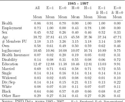
Table 7: Descriptive Statistics
1985 - 1997
All E=1 E=0 H=0 H=1 E=1 E=0
& H=1 & H=0
Mean Mean Mean Mean Mean Mean Mean
Health 0.86 0.91 0.70 0.00 1.00 1.00 0.00
Employment 0.73 1.00 0.00 0.43 0.78 1.00 0.00
Sex 0.45 0.52 0.26 0.40 0.46 0.52 0.33
Age 38.72 37.81 41.15 45.58 37.56 37.34 47.71
# Members FU 3.18 3.15 3.26 3.15 3.18 3.14 3.09
Own 0.58 0.61 0.49 0.50 0.59 0.62 0.46
log(Income) 10.65 10.86 10.08 10.07 10.74 10.89 9.75
Health Insurance 0.07 0.02 0.20 0.19 0.05 0.02 0.31
Disability 0.14 0.08 0.31 0.55 0.08 0.06 0.72
Education 12.47 12.88 11.38 10.46 12.81 13.03 9.91
Married 0.69 0.71 0.63 0.58 0.71 0.72 0.55
Single 0.14 0.14 0.16 0.14 0.14 0.14 0.14
Widowed 0.03 0.02 0.05 0.08 0.02 0.01 0.10
Div/Sep 0.14 0.14 0.15 0.21 0.13 0.13 0.22
White 0.08 0.07 0.10 0.11 0.07 0.07 0.11
Black 0.64 0.66 0.57 0.49 0.66 0.68 0.47
Other Race 0.29 0.27 0.34 0.41 0.27 0.26 0.41
Source: PSID Data, waves 1985 - 2007 E=1: Employed; E=0: Non-employed H=1: Healthy; H=0: Unhealthy
1985 - 1997
Coef. S.E. 95% Conf. Interval
HEALTH
Health0 0.4251*** (0.0166) (0.3926. 0.4577)
Healtht−2 1.1770*** (0.0152) (1.1472. 1.2068)
Employmentt−2 0.0076 (0.0148) (-0.0215. 0.0367)
log(Income) 0.0151** (0.0069) (0.0015. 0.0286)
Sex 0.0297** (0.0126) (0.0051. 0.0543)
Age -0.0395*** (0.0056) (-0.0505. -0.0285)
Age2
0.0002*** (0.0000) (0.0001. 0.0003)
Education 0.0278 (0.0262) (-0.0236. 0.0791)
Disability -0.7946*** (0.0196) (-0.8330. -0.7562)
Single -0.0289 (0.0545) (-0.1357. 0.0779)
Widowed 0.0386 (0.0690) (-0.0966. 0.1738)
Div/Sep 0.0204 (0.0348) (-0.0478. 0.0885)
White 0.1619*** (0.0267) (0.1094. 0.2143)
Black -0.0776*** (0.0272) (-0.1310. -0.0242)
# Members FU 0.0134 (0.0088) (-0.0037. 0.0306)
Own 0.0364 (0.0265) (-0.0155. 0.0884)
Health Insurance -0.0676** (0.0310) (-0.1285. -0.0068)
Healthinsrur -0.0078 (0.0458) (-0.0976. 0.0819)
Disability -0.5113*** (0.0305) (-0.5711. -0.4515)
Single -0.0305 (0.0598) (-0.1477. 0.0867)
W idowed -0.0789 (0.0806) (-0.2369. 0.0791)
Divsep -0.1327*** (0.0417) (-0.2144. -0.0509)
#M embersF U -0.0562*** (0.0102) (-0.0761. -0.0362)
Own 0.0247 (0.0320) (-0.0381. 0.0874)
log(income) 0.0858*** (0.0109) (0.0645. 0.1071)
Education 0.0356 (0.0264) (-0.0161. 0.0874)
Age 0.0103** (0.0041) (0.0022. 0.0184)
1987 0.0569* (0.0300) (-0.0019. 0.1157)
1988 0.2132*** (0.0316) (0.1513. 0.2750)
1989 0.0689** (0.0315) (0.0072. 0.1306)
1990 0.0904*** (0.0327) (0.0264. 0.1544)
1991 0.0719** (0.0316) (0.0100. 0.1338)
1992 0.0620* (0.0333) (-0.0032. 0.1272)
1993 0.0823** (0.0353) (0.0132. 0.1515)
1994 0.1183*** (0.0390) (0.0418. 0.1947)
1995 0.1865*** (0.0396) (0.1088. 0.2641)
1996 0.1247*** (0.0418) (0.0427. 0.2067)
1996 0.1850*** (0.0462) (0.0945. 0.2756)
α1 -0.8477*** (0.1179) (-1.0788. -0.6167)
continued from previous page
1985 - 1997
Coef. S.E. 95% Conf. Interval
EMPLOYMENT
Employment0 0.3371*** (0.0124) (0.3129. 0.3614)
Healtht−2 0.0508*** (0.0164) (0.0187. 0.0829)
Employmentt−2 1.4996*** (0.0118) (1.4764. 1.5227)
log(Income) 0.0314*** (0.0061) (0.0195. 0.0434)
Sex 0.3617*** (0.0110) (0.3402. 0.3831)
Age 0.0672*** (0.0046) (0.0583. 0.0762)
Age2
-0.0012*** (0.0000) (-0.0013. -0.0011)
Education 0.0310 (0.0220) (-0.0121. 0.0740)
Disability -0.3984*** (0.0199) (-0.4373. -0.3595)
Single 0.0491 (0.0434) (-0.0360. 0.1342)
Widowed -0.0255 (0.0655) (-0.1538. 0.1028)
Div/Sep 0.0573* (0.0301) (-0.0017. 0.1163)
# Members FU -0.0345*** (0.0078) (-0.0498. -0.0193)
Own 0.0054 (0.0214) (-0.0365. 0.0473)
Health Insurance -0.4904*** (0.0291) (-0.5473. -0.4334)
Healthinsrur -0.2675*** (0.0437) (-0.3532. -0.1818)
Disability -0.2642*** (0.0299) (-0.3227. -0.2056)
Single 0.1580*** (0.0482) (0.0634. 0.2525)
W idowed 0.3240*** (0.0772) (0.1726. 0.4754)
Divsep 0.2505*** (0.0366) (0.1787. 0.3223)
#M embersF U 0.0034 (0.0090) (-0.0143. 0.0210)
Own 0.0583** (0.0265) (0.0064. 0.1102)
log(income) 0.1639*** (0.0096) (0.1450. 0.1827)
Education -0.0211 (0.0221) (-0.0645. 0.0223)
Age 0.0193*** (0.0036) (0.0123. 0.0262)
1987 0.1149*** (0.0257) (0.0646. 0.1653)
1988 0.0845*** (0.0261) (0.0334. 0.1356)
1989 0.1120*** (0.0268) (0.0595. 0.1645)
1990 0.1257*** (0.0278) (0.0713. 0.1802)
1991 0.0757*** (0.0271) (0.0225. 0.1288)
1992 0.0695** (0.0285) (0.0137. 0.1254)
1993 0.1133*** (0.0302) (0.0540. 0.1725)
1994 0.2055*** (0.0334) (0.1401. 0.2709)
1995 0.2519*** (0.0338) (0.1857. 0.3181)
1996 0.2134*** (0.0357) (0.1434. 0.2834)
1997 0.2565*** (0.0391) (0.1799. 0.3331)
α2 -4.3527*** (0.0977) (-4.5441. -4.1614)
/athrho 0.0835*** (0.0095) (0.0648. 0.1022)
Table 9: Marginal effects. Sample: 1985 - 1997
Sample: 1985 - 1997
P r(H = 1, E= 1) P r(H= 1, E= 0) P r(H = 0.E = 1) P r(H= 0.E= 0) P r(H = 1) P r(E= 1) ∂Y
∂X S.E.
∂Y
∂X S.E.
∂Y
∂X S.E.
∂Y
∂X S.E.
∂Y
∂X S.E.
∂Y
∂X S.E.
Healtht−2 0.1354*** (0.0047) 0.0238*** (0.0042) -0.1213*** (0.0020) -0.0378*** (0.0010) 0.1591*** (0.0024) 0.0140*** (0.0045)
Employmentt−2 0.3820*** (0.0037) -0.3810*** (0.0034) 0.0324*** (0.0017) -0.0334*** (0.0008) 0.0010 (0.0020) 0.4144*** (0.0035)
log(Income) 0.0096*** (0.0017) -0.0075*** (0.0016) -0.0009 (0.0007) -0.0012*** (0.0003) 0.0020** (0.0009) 0.0087*** (0.0017) Sex 0.0950*** (0.0031) -0.0910*** (0.0028) 0.0049*** (0.0013) -0.0089*** (0.0005) 0.0040** (0.0017) 0.0999*** (0.0030) Age 0.0130*** (0.0013) -0.0183*** (0.0012) 0.0056*** (0.0006) -0.0003 (0.0002) -0.0053*** (0.0008) 0.0186*** (0.0013) Age2 -0.0003*** (0.0000) 0.0003*** (0.0000) 0.0000*** (0.0000) 0.0000*** (0.0000) 0.0000*** (0.0000) -0.0003*** (0.0000) Education 0.0108* (0.0063) -0.0070 (0.0056) -0.0022 (0.0028) -0.0015 (0.0010) 0.0038 (0.0035) 0.0086 (0.0061) Disability -0.1839*** (0.0056) 0.0765*** (0.0051) 0.0738*** (0.0022) 0.0336*** (0.0010) -0.1074*** (0.0027) -0.1101*** (0.0055) Single 0.0092 (0.0124) -0.0132 (0.0108) 0.0042 (0.0060) -0.0002 (0.0020) -0.0040 (0.0076) 0.0134 (0.0117) Widowed -0.0028 (0.0187) 0.0079 (0.0174) -0.0044 (0.0068) -0.0007 (0.0026) 0.0051 (0.0088) -0.0072 (0.0187) Div/Sep 0.0165** (0.0084) -0.0138* (0.0075) -0.0009 (0.0036) -0.0018 (0.0012) 0.0027 (0.0046) 0.0156* (0.0081) White 0.0169*** (0.0031) 0.0051*** (0.0009) -0.0169*** (0.0031) -0.0051*** (0.0009) 0.0220*** (0.0040) (omitted)
Black -0.0096*** (0.0032) -0.0028*** (0.0010) 0.0096*** (0.0032) 0.0028*** (0.0010) -0.0124*** (0.0042) (omitted)
# Members FU -0.0074*** (0.0022) 0.0092*** (0.0020) -0.0022** (0.0009) 0.0003 (0.0003) 0.0018 (0.0012) -0.0095*** (0.0021) Own 0.0052 (0.0062) -0.0002 (0.0055) -0.0037 (0.0028) -0.0013 (0.0010) 0.0049 (0.0036) 0.0015 (0.0059) Health Insurance -0.1317*** (0.0082) 0.1226*** (0.0075) -0.0038 (0.0033) 0.0130*** (0.0012) -0.0091** (0.0042) -0.1355*** (0.0081)
Source: Self Calculations *p < .1; **p < .05; ***p < .01
Table 10: Coefficients and Standard Errors obtained from the univariate probit estimations of Specifications 2 and 3
Sample: 1985 - 2007(Odd Years)
Specification 2 Specification 3
Health Employment Health Employment
Coef. S.E. Coef. S.E. Coef. S.E. Coef. S.E. Health0 0.3200*** (0.0195)
Employment0 0.2004*** (0.0136)
Healtht−2 1.1301*** (0.0173) 0.1067*** (0.0175) 1.3122*** (0.0156) 0.1489*** (0.0169)
Employmentt−2 0.0037 (0.0161) 1.2922*** (0.0129) 0.0654*** (0.0156) 1.3954*** (0.0118)
log(Income) 0.0105 (0.0075) 0.1053*** (0.0064) 0.0555*** (0.0057) 0.1600*** (0.0050) Sex 0.0366*** (0.0137) 0.3917*** (0.0118) 0.0364*** (0.0135) 0.4111*** (0.0115) Age -0.0333*** (0.0051) 0.1092*** (0.0041) -0.0345*** (0.0045) 0.1044*** (0.0036) Age2
0.0002*** (0.0001) -0.0014*** (0.0000) 0.0002*** (0.0001) -0.0014*** (0.0000) Education 0.0256 (0.0180) 0.0759*** (0.0158) 0.0749*** (0.0029) 0.0263*** (0.0025) Disability -0.8201*** (0.0212) -0.5489*** (0.0206) -1.0502*** (0.0151) -0.6591*** (0.0149) Single 0.0256 (0.0524) 0.1759*** (0.0415) -0.0471** (0.0226) 0.0860*** (0.0186) Widowed 0.1171* (0.0666) 0.1103* (0.0615) -0.0751** (0.0376) 0.1700*** (0.0356) Div/Sep 0.0642* (0.0331) 0.0668** (0.0282) -0.0620*** (0.0195) 0.1460*** (0.0172) White 0.1566*** (0.0334) 0.1701*** (0.0329)
Black -0.0970*** (0.0337) -0.1150*** (0.0332)
# Members FU 0.0196** (0.0084) -0.0492*** (0.0072) -0.0155*** (0.0049) -0.0541*** (0.0042) Own 0.0325 (0.0254) 0.0171 (0.0207) 0.1116*** (0.0157) 0.1213*** (0.0132) Health Insurance -0.0639*** (0.0240) -0.1738*** (0.0212) -0.0186 (0.0190) -0.1458*** (0.0172)
Insurance 0.1636*** (0.0385) 0.1022*** (0.0334)
Disability -0.4774*** (0.0338) -0.2253*** (0.0316)
Single -0.0582 (0.0585) -0.0031 (0.0469)
W idowed -0.2028** (0.0850) 0.1686** (0.0791)
divsep -0.1506*** (0.0423) 0.1948*** (0.0365)
#M embersF U -0.0581*** (0.0103) -0.0002 (0.0089)
Own 0.0683** (0.0330) 0.1202*** (0.0277)
log(Income) 0.1004*** (0.0122) 0.1239*** (0.0106)
Education 0.0360** (0.0183) -0.0653*** (0.0160)
Age 0.0025 (0.0028) -0.0019 (0.0025)
1989 0.0332 (0.0306) -0.0256 (0.0252) 0.0493* (0.0297) -0.0179 (0.0246) 1991 0.0460 (0.0315) -0.0608** (0.0259) 0.0719** (0.0298) -0.0465* (0.0245) 1993 -0.0051 (0.0310) -0.1007*** (0.0258) 0.0125 (0.0279) -0.0816*** (0.0233) 1995 0.0702** (0.0342) 0.0230 (0.0285) 0.1096*** (0.0300) 0.0475* (0.0249) 1997 0.0234 (0.0372) -0.0316 (0.0312) 0.0823** (0.0319) 0.0051 (0.0262) 1999 0.0441 (0.0376) 0.1252*** (0.0321) 0.0784** (0.0341) 0.1426*** (0.0291) 2001 0.0302 (0.0395) 0.0554 (0.0338) 0.0707** (0.0338) 0.0755*** (0.0287) 2003 -0.0187 (0.0411) 0.1052*** (0.0356) 0.0251 (0.0330) 0.1297*** (0.0284) 2005 -0.0709 (0.0431) 0.1268*** (0.0375) -0.0219 (0.0324) 0.1549*** (0.0282) 2007 -0.0301 (0.0455) 0.1172*** (0.0395) 0.0296 (0.0321) 0.1464*** (0.0278)
Table 11: Marginal effects. Sample: 1985 - 2007 (Odd Years) Specifications 2 and 3
Sample: 1985 - 2007(Odd Years)
Specification 2 Specification 3
P r(H = 1) P r(E = 1) P r(H = 1) P r(E = 1)
∂Y
∂X S.E.
∂Y
∂X S.E.
∂Y
∂X S.E.
∂Y
∂X S.E.
Healtht−2 0.1512*** (0.0027) 0.0280*** (0.0046) 0.1788*** (0.0026) 0.0392*** (0.0044)
Employmentt−2 0.0005 (0.0022) 0.3387*** (0.0036) 0.0089*** (0.0021) 0.3672*** (0.0034)
log(Income) 0.0014 (0.0010) 0.0276*** (0.0017) 0.0076*** (0.0008) 0.0421*** (0.0013)
Sex 0.0049*** (0.0018) 0.1027*** (0.0031) 0.0050*** (0.0018) 0.1082*** (0.0030)
Age -0.0045*** (0.0007) 0.0286*** (0.0011) -0.0047*** (0.0006) 0.0275*** (0.0009)
Age2
0.0000*** (0.0000) -0.0004*** (0.0000) 0.0000*** (0.0000) -0.0004*** (0.0000)
Education 0.0034 (0.0024) 0.0199*** (0.0041) 0.0102*** (0.0004) 0.0069*** (0.0006)
Disability -0.1098*** (0.0029) -0.1439*** (0.0054) -0.1431*** (0.0023) -0.1734*** (0.0040)
Single 0.0034 (0.0069) 0.0439*** (0.0097) -0.0065** (0.0032) 0.0225*** (0.0047)
Widowed 0.0147* (0.0077) 0.0284* (0.0151) -0.0105* (0.0055) 0.0428*** (0.0083)
Div/Sep 0.0084** (0.0042) 0.0175** (0.0073) -0.0086*** (0.0028) 0.0371*** (0.0042)
White 0.0209*** (0.0049) 0.0230*** (0.0049)
Black -0.0155*** (0.0051) -0.0189*** (0.0052)
# Members FU 0.0026** (0.0011) -0.0129*** (0.0019) -0.0021*** (0.0007) -0.0142*** (0.0011)
Own 0.0043 (0.0034) 0.0045 (0.0054) 0.0152*** (0.0021) 0.0319*** (0.0035)
Health Insurance -0.0085*** (0.0032) -0.0456*** (0.0056) -0.0025 (0.0026) -0.0384*** (0.0045)
Source: Self Calculations *p < .1; ** p < .05; ***p < .01