M
aster
T
hesis
Credit Spreads and Monetary
Policy in a Small Open Economy:
an Analysis of the Colombian
Economy
Author:
Alexander B
allesteros
Supervisor:
Jesus B
ejarano
A thesis submitted in fulfillment of the requirements
for the degree of Master in Economics
Policy in a Small Open Economy:
an Analysis of the Colombian
Economy
alexander ballesteros
abstract
This paper estimates Bejarano and Charry (2014)’s small open economy
with financial frictions model for the Colombian economy using Bayesian estimation techniques. Additionally, I compute the welfare gains of implementing an optimal response to credit spreads into an augmented Taylor rule. The main result is that a reaction to credit spreads does not imply significant welfare gains unless the economic disturbances increases its volatility, like the disruption implied by a financial crisis. Otherwise its impact over the macroeconomic variables is null.
1 introduction
The2008financial crisis renewed economists’ interest over the debate about the role of central banks on the achievement financial stability. In this de-bate, whether monetary authority should target a financial measure besides inflation and output to prevent a negative impact over the economy has gained importance.
Motivated by Taylor (2008) and Mishkin (2008), which proposed that the Federal Reserve should lower the interest rate to increases of credit spreads as a way to mitigate the adverse effect of the financial crisis over the real economy, Curdia and Woodford (2010) analyzed the effects of including the spread between deposits and loans interest rate into a Taylor Rule in a DSGE framework calibrated to reflect US economy dynamics . They found that this reaction is recommended for financial and non-financial disturbances, but the optimal size of the response would depend on the source and the persistence of the disturbance. Additionally, empirical studies such as Belke and Klose (2010), Castro (2011), Martin and Milas (2013), and Huang (2015) have concluded that the Federal Reserve, the European Central Bank or the Bank of England have responded to credit spreads during or before the2008
financial crisis.
These studies were focused mainly on developed economies. However, analysis of the relation between monetary policy and credit spreads are scarce in countries like Colombia. Since Colombian monetary policy is conducted similarly to US, it is possible to apply Curdia and Woodford
(2010) analysis to the Colombian framework. However, US and Colombian economies differ in several aspects; mainly that Colombia is a small open economy.
In this sense, Bejarano and Charry (2014) extended Curdia and Woodford (2010) model to a small open economy framework. Their conclusions differ substantially from Curdia and Woodford (2010) model since they found that including spreads on the Taylor rule is just recommended if the source of the disturbance is the foreign interest rate. An important remark about Bejarano and Charry (2014) model is that most of the parameters used were the same as Curdia and Woodford (2010) analysis in order to focus mainly on the effect of opening the economy.
In order to apply this analysis to the Colombian economy, this paper es-timates Bejarano and Charry (2014) model’s structural parameters through Bayesian estimation techniques using Colombian data on main macroeco-nomic variables, as on interest rates. The main reason to estimate the struc-tural parameters using Colombian data is for the model to reflect Colombian aggregate variables dynamics. Both, Curdia and Woodford (2010) and Be-jarano and Charry (2014) conclusions are based on a calibration that reflects US macroeconomics variable dynamics, but these conclusions might differ in the context of the Colombian economy.
Once the parameters are estimated, this paper computes the optimal re-sponse to credit spreads in a Taylor rule by maximizing an aggregate welfare function approximated up to second order. Then, to asses the gains of im-plementing the optimal response described above, we compute the welfare loss as the percentage of consumption sacrificed from not reacting at all to credit spreads instead of implementing the optimal reaction. Finally, we perform counterfactual analysis comparing historic data to simulated data where monetary authority implements the optimal response. This is done to to determine the impact on macroeconomic variables, such as output or debt, of implementing the optimal reaction.
The main result of this research is that implementing an optimal reac-tion to credit spreads do not imply significant welfare gains because credit spreads volatility is low compared to other macroeconomic variables. The Credit spread is rather a stable measure that does not have great impact over the economy. If the the central bank implemented an optimal response to credit spread, aggregate macroeconomic variables would display almost exactly the same dynamics as if it did not respond at all. However, similar to the2008 financial crisis, during financial turmoil credit spreads volatil-ity increases significantly and impacts adversely debt and output. In this scenario, it is highly recommended to react to credit spreads as it would stabilize output faster and prevent it from falling that much compared to not reacting at all.
2 a small open economy with financial frictions
This is a basic New Keynesian model with the following additional as-sumptions: i) the existence of two different types of households: savers and borrowers, ii) the economy can only channel funds from savers to bor-rowers through a financial intermediary, iii) the financial intermediary can be funded by foreign liabilities, besides savers funds, and iv) households can consume three different baskets: domestic traded goods, domestic non-traded goods, and imported goods. The first two assumptions account for the introduction of a financial friction that creates a wedge between the de-posit and the credit interest rate. The last two account for setting the small open economy framework.
2.1 Financial Friction: the Credit Spread
2.1.1 Heterogeneous Households: Intertemporal Optimization Problem
Heterogeneity is introduced by assuming that households differ in their preferences. Hence, at period t they can be either a saver or a borrower household according to the following discounted intertemporal objective function:
E0 ∞
∑
t=0
βt
uτt(i)(c
t(i);εt)− Z 1
0 v
τt(i)(h
t(j;i);εt)dj
(1)
where τt(i)∈ {b,s}indicates the household’s type in periodt. Period
util-ityuτt(i)(ct(i);εt)is function of a Dixit-Stiglitz aggregator of differentiated
consumption goodsct(i). Disutility of workvτt(i)(ht(j;i);εt)is function of a
continuum of different types of specialized labor, indexed byj, that house-holds supply to domestic non-traded good firms. Finally, both uτt(i) and
vτt(i)can be shifted by a vector of aggregate taste shocksεt.
For this analysis we assume that utility of consumption and disutility of work are of the form:
uτt(i)(c
t(i);εt) = ct(i) 1−1
στC¯τστ1
1− 1
στ
(2)
and
vτt(i)(h
t(j;i);εt) = ψτ
1+νht(i,j)
1+νH¯
t−ν (3)
where στ is the intertemporal elasticity of substitution of type τ; ¯Cτ
t is an
aggregate preference shock to consumption of typeτ;ψτ is a scalar factor for type τ, ν is the inverse Frisch elasticity of labor supply, and ¯Ht is an
aggregate preference shock to labor.
Households may change type according to an independent two-state Markov chain. Each period, with probability 1−δeach household may drawn a new type; otherwise it remains the same. After a new type is drawn, it becomes a borrower with probabilityπband a saver with probabilityπs. It is assumed
risk-sharing households that can sign state contingent contracts with one an-other to insure against aggregate and idiosyncratic risk from the household random drawn of its type.1 This insurance is intermittent, and households
are only able to sign these contracts whenever they face a new type drawn. In this case, household will receive a net transfer Tt(i) and learns its type.
Then, it makes its spending, saving and borrowing decisions, taking into account its new type.
Household’s beginning-of-period nominal net financial wealth is given by:
At(i) = [Bt−1(i)]+(1+idt−1) + [Bt−1(i)]−(1+itb−1) +Dintt +Tt(i) (4)
where Bt−1 is the household net financial wealth for period t−1; [B]+ ≡
max(B, 0)is the financial wealth household i has on deposits to the finan-cial intermediaries or government debt; [B]− ≡ min(B, 0) if the financial wealth from credit owed to the financial intermediaries; idt is the riskless one-period deposits interest rate,ibt is the borrowing interest rate; andDintt
is the distributed profits from the financial intermediary.
Households end-of-period nominal net financial wealth is given by:
Bt(i) =At(i)−Ptct(i) + Z j
0 Wt(j)ht(i,j)dj+Dn,t+Dx,t+Dm,t+T g t (5)
where Pt is the Dixit-Stiglitz price index for periodt;Wt(j) is the wage of
labor typej;Dn,tare the profits from the non-traded good producing firms;
Dx,t are the profits from the traded good producing firms; Dm,t are the
profits from the imported good producing firms; and Ttg is the lump-sum transfer received from the government.
If it is assumed thatψs andψbare calibrated so that both types choose to
work the same hours in steady state, the existence of heterogeneous house-holds is guaranteed, at least around the equilibrium, ifubc(c;ε)>usc(c;ε)(so borrowers have a higher impatience to consume) andibt >idt. The fist condi-tion is assured by calibratingσb >σs, the second will be shown in the next
section. These two conditions imply that the set of borrowersBwill always chooseBt(i)<0, the set of saversSwill chooseBt(i)>0, andi= [B,S].2
By maximizing (1) with respect toct(i), ht(i,j), and Bt(i)/Pt subject to
(4) and (5) and, then, aggregating overBand Swe have the following fist order conditions:
λτt =
C¯τ
t
cτ
t
1 στ
(6)
µwt ψτ
ht(j)τ
¯
Ht
ν
=λτt
Wt(j)
Pt (7)
λst=βEt
(
(1+idt)
Πt+1 [δλ
s
t+ (1−δ)Λt]
)
(8)
λbt =βEt
(
(1+ib t)
Πt+1 h
δλbt+ (1−δ)Λt
i)
(9)
Λt=πbλst+πsλbt (10)
whereλτt is the marginal utility of consumption for typeτ,Λtis the marginal utility aggregated over i , µwt is a wage mark-up shock which is assumed exogenous, andΠt=Pt/Pt−1is periodtinflation.
2.1.2 Financial Intermediaries
As it was stated above, when households cannot sign state-contingent con-tracts, we assume that funds from savers to borrowers can only be channeled through a financial intermediary. Additionally, we assume that the financial intermediary can also channel funds to borrowers from international finan-cial markets.3 Then, expected real profits from the financial intermediary sector can be expressed as 4
Et
Dintt+1 Pt+1 =Et
(
bt(1+itb)
Πt+1 −
dt(1+itd)
Πt+1 −qt+1b ∗
t(1+idt∗)(1+ϕt)
) (11)
where bt are the aggregate loans, dt are the aggregate deposits, qt is the
real exchange rate, b∗t are international financial markets funds, idt∗ is the
foreign interest rate, which is assumed to be exogenous, and ϕt is the risk
premium with the form suggested by Schmitt-Grohe and Uribe (2003) where it increases to deviations of international financial markets funds to GDP ratio from its steady state value:
ϕt=ψ1
exp(qtbt
gdpt−
qssbss
gdpss)−1
(12)
The financial intermediary can only channel these funds assuming a cost Ξ(bt) and faces an aggregate default probability χt on every loan, which
is assumed exogenous. We assume that the costs associated to channeling funds come from consuming non-traded goods. In order to repay savers and international financial markets we have the following real resource con-straint for financial intermediaries:
bt+gPn,tΞ(bt) +χtbt=dt+qtb∗t (13)
wheregPn,t=Pn,t/Ptis the non-traded good price relative to the Dixit-Stiglitz
price index. We assume thatΞ(bt) =Ξetbηt , withη>1 in order to have non-decreasing and convex cost over aggregate loans, and we assumeΞetto be an exogenous shock. By maximizing (11) with respect tobt,dt, andb∗t subject
to (13) we have that:
(1+itb) = (1+idt)(1+ωt) (14)
(1+idt) =Et
(
qt+1(1+itd∗)(1+ϕt)Πt+1
qt
)
(15)
where ωt is the credit spread from deposits and loans interest rate of the
form:
ωt=gPn,tΞetηbηt−1+χt (16)
As it was discussed above, one condition to guarantee the existence of heterogeneous households was thatibt >id
t, which we make sure since from
the definitionωt>0.
3 We calibrate the model in order that financial intermediaries always choose to borrow from international markets instead of lending them; henceb∗
t >0.
2.2 The Small Open Economy
2.2.1 Intratemporal Optimization Problem
Another important characteristic of a Small Open Economy is for the possi-bility to import a foreign traded-good and to export a domestic traded good. In this sense, it is assumed that the Dixit-Stiglitz aggregator of differentiated consumption goodsct(i)is of the form:
ct(i) =
γρ1hc
h,t(i)
ρh−1
ρh + (1−γ)ρ1hc
f,t(i)
ρh−1 ρh
ρh ρh−1
(17)
where γ is the parameter controlling the participation of households ex-penditure in domestic goods, ρh is the elasticity of substitution between
imported and domestic goods consumption,ch,t(i)is householdi
consump-tion of the domestic good, and cf,t(i) is households i consumption of the
imported good.
Additionally, the consumption of the domestic good can be differentiated between the consumption of a non-traded good and a traded good by
ch,t(i) =
γ
1 ρn n cn,t(i)
ρn−1
ρn + (1−γn) 1 ρncx,t(i)
ρn−1 ρn
ρn ρn−1
(18)
where, similarly as above, γn controls the participation of household
con-sumption in the domestic non-traded good, ρn is the elasticity of
substitu-tion between the domestic non-traded good and the domestic traded good,
cn,t(i) is household i consumption of the domestic non-traded good, and
cx,t(i)is householdsiconsumption of the domestic traded good.
We assume that the domestic non-traded good and the imported good are baskets of differentiated goods indexed byjandm, respectively. Then it follows that:
cn,t(i) =
Z 1
0 cn,t(j)
θn−1 θn dj
θn θn−1
(19)
cf,t(i) =
"Z
1
0 cf,t(m)
θf−1 θf
dm
# θf θf−1
(20)
Since household heterogeneity has no impact over the optimal composi-tion of consumpcomposi-tion baskets, we can aggregate overiand solve households intra-temporal consumption decision problems. This will provide us with the following equilibrium conditions:
• For the optimal allocation between domestic and imported goods
ch,t=γctgPh,t
−ρh
(21)
cf,t= (1−γ)ctgPf,t
−ρh
(22)
Pt=
h
γP1−ρh
h,t + (1−γ)P 1−ρh f,t
i 1 1−ρh
• For the optimal allocation between domestic non-traded and traded goods
cn,t=γnch,tPn,t−ρn (24)
cx,t= (1−γn)ch,tPx,t−ρn (25)
Ph,t=
h
γnPn,t1−ρn+ (1−γn)Px,t1−ρn
i 1 1−ρn
(26)
WherePn,t=Pn,t/Ph,tand Px,t=Px,t/Ph,t.
• For the optimal allocation between differentiated domestic non-traded goods
cn,t(j) =
Pn,t(j)
Pn,t
−θn
cn,t (27)
Pn,t=
Z 1
0 Pn,t(j)
θn−1dj
1 θn−1
(28)
• For the optimal allocation between differentiated imported goods
cf,t(m) =
Pf,t(m)
Pf,t
!−θf
cf,t (29)
Pf,t=
Z 1
0 Pf,t(m)
θf−1dm
1 θf−1
(30)
2.2.2 Firms’ Pricing Decision Domestic Non-Traded Good
We assume that households supply labor to eachjnon traded good produc-ing firms. From equation (7) we can solve for hτt and aggregate overi to obtain labor supply to firmj
ht(j) =H¯t
"
Wt(j)
Pt
e
λt
µwtψ
#1 ν
(31)
where
e
λt
ψ
!1 ν
=πb
λbt ψb
!1 ν
+πs
λst ψs
1 ν
(32)
Additionally, we assume that non-traded good producing firms have a production technology of the form:
yn,t(j) =zt(ht(j))
1
φ (33)
whereztis a productivity shock common to all non-traded good producing
firms, andφis assumed to be grater than1. We define labor real expenditure of firmjas:
linct(j) = Wt(j)
Pt
Given thatyn,t(j) =cn,t(j), and replacing equation (27), we can determine
linct(j)by solving forht(j)in equation (33) andWt(j)/Ptin equation (31).
Then, we have that:
linct(j) = µ w tψ
e
λtH¯tν
!
yn,t
zt
1+ωyP n,t(j)
Pn,t
−θn(1+ωy)
(35)
whereωy=φ(1+ν). We can define firmjnominal profits as
Dn,t(j) = [Pn,t(j)yn,t(j)(1−τn,t)−Ptlinct(j)] (36)
where τn,t is the tax payed for each sold non-traded good. Firmjcan only
update its pricePn,t(j)with probabilityαeach period. Then, replacing
equa-tions (27), (33), and (35), firm jmaximizing problem becomes:
Pn,t(j)∗=argmax
"
Et ∞
∑
T=t
αT−tQt,T
(
Pn,t(j)
Pn,t(j)
Pn,T
−θn
yn,T(1−τn,T)−
PT
µwTψ
f
λTH¯νT
! y
n,T
zT
1+ωyP n,t(j)
Pn,T
−θn(1+ωy))#
(37)
WhereQt,T is the stochastic discount factor given by
Qt,T =βT−t
ΛTPt
ΛtPT (38)
From the maximization problem stated above we get the following fist order condition:
Pn,t(j)∗
Pn,t
θnωy+1
= Kn,t
Fn,t (
39)
Where
Kn,t=Λtµn(1+ωy) µ w tψ
e
λtH¯tν
! y
n,t
zt
1+ωy
+αβEt[Kn,t+1Π
θn(1+ωy) n,t+1 ] (40)
Fn,t=ΛtgPn,tyn,t(1−τn,t) +αβEt[Fn,t+1Πn,tθn−+11] (41)
Here Kn,t is the discounted marginal cost, µn = θn/(θn−1) is the firm’s
mark up, Πn,t is the non-traded good inflation, and Fn,t is the discounted marginal revenue. Because only a shareαof all non-traded good producing firms can update their prices, we replace equation (39) in (28), aggregate overj, and, after some algebra, get
Πn,t=
1−(1−α)Kn,t Fn,t
1−θn 1+θnωy
α 1 θn−1
Imported Good
We assume that an importing firm can differentiate an imported good at no cost and then sell it to the households. Then, firm m nominal profits are given by
Df,t(m) =
h
Pf,t(m)yf,t(m)(1−τf,t)−StP∗f,tyf,t(m)
i
(43)
where St is the nominal exchange rate,τf,t is a tax for each imported good
sold, and P∗f,t is the imported good international price, which is assumed exogenous. Similarly to the non-traded good producing firms, they can only update its price with probability α each period. Since cf,t(m) = yf,t(m),
replacing equation (29) into equation (43), firm m maximizing problem becomes:
Pf,t(m)∗ =argmax
Et
∞
∑
T=t
αT−tQt,T
Pf,t(m)
Pf,t(m)
Pf,T
!−θf
yf,T(1−τf,T)−
StP∗f,t
Pf,t(m)
Pf,t
!−θf
cf,t
(44)
From this maximization problem we get the following fist order condition:
Pf,t(m)∗
Pf,t
!
= Kf,t
Ff,t
(45)
Where
Kf,t=ΛtµfqtP∗f,tyf,t+αβEt[Kf,t+1Π
θf
f,t+1] (46)
Ff,t=ΛtgPf,tyf,t(1−τf,t) +αβEt[Ff,t+1Π
θf−1
f,t+1] (47)
Here Kf,t is the discounted marginal cost, µf = θf/(θf −1) is the firm’s
mark up, Πf,t is the imported good inflation, and Ff,t is the discounted
marginal revenue. Similarly to the non-traded good case, by replacing equa-tion (45) into (30), and aggregating overmwe get
Πf,t=
1−(1−α)Kf,t Ff,t
1−θf
α
1 θf−1
(48)
Domestic Traded Good
Finally, we assume that the domestic traded good price is set abroad. Hence, the price that households pay for the domestic traded good can be described by
g
Px,t=qtPx,t∗ (49)
where gPx,t = Px,t/Ptand Px,t∗ is the domestic traded price payed at
that the domestic economy is endowed withyx,tunits of the domestic traded
good, then domestic traded good firm profits is described by:
Dx,t=gPx,tyx,t(1−τx,t) (50)
where τx,t is a tax charged by the government for every unit of domestic
traded good produced.
2.2.3 Aggregate Supply
Given that the domestic non traded good is used by households, govern-ment expenditure and the financial intermediary in order to channel funds to borrowers, aggregate domestic non-traded good can be expressed as
yn,t=cn,t+gt+Ξtbηt (51)
At the same time, the domestic traded good is exported, so the the firms produce this to satisfy domestic and foreign demand given by
yx,t=cx,t+c∗x,t (52)
where c∗x,t corresponds to exports of the domestic traded good, which is assumed exogenous. Finally, firms import the foreign good just in order to satisfy domestic demand. This implies
yf,t=cf,t (53)
Using equations (51), (52), and (53) we can characterize Gross Domestic Product as
gdpt=gPn,tyn,t+gPx,tyx,t+gPf,tyf,t−qtP∗f,tyf,t (54)
2.3 Public Sector Fiscal Policy
The government is assumed to purchase quantity gt of the domestic
non-traded good. This purchase is financed by taxes to each unit sold of the domestic traded goodτx,t, the domestic non-traded goodτn,t, the imported
goodτf,t, and additionally, lump-sum taxes to householdsTtg and
borrow-ing from households at(1+idt). Hence, government’s real budget constraint is given by
g
Pn,tgt=gPx,tyx,tτx,t+gPn,tyn,tτn,t+gPf,tyf,tτf,t+b g t +
Ttg Pt −b
g t−1
(1+idt)
Πt (55)
We assume thatτx,t,τn,t,τf,t,gt, andbtgare exogenous shocks.
Monetary Policy
Following Curdia and Woodford (2010) we assume that monetary policy is represented by an augmented Taylor Rule that account for deviations of the credit spread from its steady state value besides deviations of inflation from its target value andgdptfrom its natural value. This means that the deposits
interest rate is represented as
Herein,dt and gdpnt represents the natural deposit interest rate and gross domestic product in a economy without financial frictions and flexible price setting for the domestic non-traded and imported good. 5
2.4 Aggregate Private Indebtedness Dynamics
We can see from equation (16) that the credit spread is a function of ag-gregate debt and, differently from the basic New Keynesian model, we not longer assume that in the aggregate this equates to zero. Then, it is im-portant to characterize its dynamics in order to close the model. For this purpose, we should aggregate equation (5) overB. Then we have:
Ptbt= Z
BBt(i)di=− Z
B{At(i) +Rt(i)}di (57)
The fist term is the beginning of period net financial wealth held by bor-rowers, and the second is their excess of consumption for period t given by:
Rt(i) = Z 1
0 Wt(j)ht(i,j)dj+Dn,t+Dx,t+Df,t+T g
t −Ptct(i) (58)
Borrowers Beginning of Period Net Financial Wealth is characterize by
Z
BAt(i)di=δ
n
−Pt−1bt−1(1+ibt−1) +πbDintt
o
+ (1−δ)πbAt (59)
The first term relates the beginning of period financial wealth for those who did not change type and, hence, did not receive any insurance transfer. The second term correspond to those who did receive the transfer. Aggre-gating equation (4) overiwe have that:
At=Pt−1(bt−1+bgt−1)(1+idt−1)−Pt−1bt−1(1+ibt−1) +Dintt (60)
Using the definition ofDintt from equation (11), and the uncovered inter-est parity condition from equation (11), and expressing in real terms, we have
At
Pt =
btg−1−bt∗−1qt−1
(1+id t)
Πt (61)
Then, the beginning of period financial wealth is the debt held by the government less the debt from international financial markets. Aggregating the second term in equation (57) we have
Z
BRt(i)di=πbR b t =πb
n
Wtb+Dn,t+Dx,t+Df,t+Ttg−Ptcbt
o
(62)
whereWb t =
R
B
R1
0 Wt(j)ht(j)djdiis the nominal labor income for borrowers.
For both types, we have that aggregating equation (35) overjand over each type, real labor income for each one is:
Z
τ
Z 1
0
Wt(j)
Pt ht(j)djdi=w
τ
t =
µwtψτ
λτtH¯ν
t
yn,t
zt
1+ωy
∆n,t (63)
where ∆n,t is the domestic traded good price dispersion. Following Curdia and Woodford (2009) appendix,∆n,tis expressed as
∆n,t=
Z 1
0
Pn,t(j)
Pn,t
−θn(1+ωy)
dj
=α∆n,t−1Πφ(1+ωy)
n,t + (1−α)
Kn,t
Fn,t
−φ(1+ωy)
1+ωyθ
(64)
Aggregating profit equations (36) and (43), using government budget constraint in equation (54), and expressing in real terms, we get from equa-tion (62):
πbRbt
Pt =πb
n
cbt+πs(wbt−wts) +gdpt
−gPn,tgt+btg−b g t−1
(1+idt)
Πt
) (65)
where wst is the real labor income that corresponds to savers. Replacing equations (51), (52), and (53), that characterize aggregate supply, equations (22), (24), and (25) that determine the optimal allocation for the different consumption baskets, into equation (54) we can reexpress gdptas
gdpt=ct+gPn,t(Ξtbtη+gt) +gPx,tc∗x,t−qtP∗f,tyf,t (66)
wherect=πbcbt +πscst. Finally, replacing equation (66) into (65), we get:
πbRbt
Pt =πbπs
(cbt−cst)−(wbt−wst)
+πb b g t −b
g t−1
(1+idt−1)
Πt +Tbt+gPn,tΞtb η
t
! (67)
Where,
Tbt=gPx,tc∗x,t−qtP∗f,tyf,t (68)
We can further reexpress equation (67) by finding a relation between the trade balance Tbt, and the dynamics of foreign debt. By defining
aggre-gate saving similar to equation (57) we can express financial intermediaries resource constraint in equation (13) as:
qtb∗t =b g t −
At
Pt −πb
Rbt Pt −πs
Rst Pt +
g
Pn,tΞ(bt) +χtbt (69)
Through a similar process to reach equation (67) we have that
πb
Rbt Pt +πs
Rst Pt =b
g
t +Tbt+gPn,tΞtbηt −bt−1
(1−id t−1)
Πt (70)
Replacing (66) into (65) we have that
qtb∗t =qt−1bt∗−1
(1−idt−1)
Replacing equations (59), (61), (67), and (71) into (57) we have that the dynamics of private indebtedness are characterized by the following expression
bt(1+πbωt) =δ
"
bt−1
(1−ibt−1)
Πt −πb
Dint t
Pt
#
+πb
"
qtbt∗−δqt−1bt∗−1
(1+idt−1)
Πt !
− bgt −δbtg−1(1+i
d t−1)
Πt !#
πbπs
h
(cbt−cst)−(wbt−wst)i
(72)
I can be seen, that aggregate debt depends on the beginning-of period financial wealth held by borrowers, the change of the aggregate beginning-of period financial wealth (we can see from equation (61) that the middle term is proportional to the change ofAt/Ptfrom periodt−1 tot), and the
consumption-labor income difference from borrowers to savers.
3 bayesian estimation
Since the purpose of this article is to determine the existence on any benefits to the Colombian economy from targeting credit spreads in the Taylor Rule described in equation (56), we need to set the model’s parameters to reflect Colombian aggregate variable dynamics. In order to do this we use Bayesian estimation techniques.
3.1 The Structural Parameters
First, it is useful to list the model’s parameters. This is is a model with15 ex-ogenous shock that, as described above, come from the following variables:
¯
Cb
t, ¯Cts, ¯Ht,µwt,itb∗,Ξet,χt,zt,P∗f,t,Px,t∗ ,c∗t,τn,t,τf,t,gt,bgt.6 We assume that each
one follows an independent AR(1) process; so this means that we would have30 parameters related to the exogenous processes accounting for the autoregressive and the standard error parameters. Additionally, the model has23structural parameters which are listed below:
Table1: Structural Parameters
1. σb 2. σs 3. ν 4. ψb 5. ψs 6. ψ 7. δ 8. πb 9. πs 10. ψ1 11. η 12. γ 13. ρh 14. γn 15. ρn 16. θn 17. θf 18. φ 19. α 20. β
21. φΠ 22. φy 23. φω
Differently from most Real Business Cycle models, the steady state de-posits interest rate no longer reflect the inverse ofβ. Now it has to account
[image:14.595.140.490.122.215.2]for the both types of interest rates. In this sense, we can solveβfrom equa-tions (8) and (9), which would be calibrated to
β= δ+1+ωss(δ+ (1−δ)πb)−
p
(δ+1+ωss(δ+ (1−δ)πb))2−4δ(1+ωss) 2idssδ(1+ωss)
(73)
As it was stated above,ψbandψsare calibrated in order to equate worked
hours for both types in steady state. Since wages are the same for both types of households, we can see from equation (72) and (63) that equating worked hours is the same as equating real labor income for both types. This implies that
ψb
ψs =
λbss
λs ss
=Ω (74)
If equation (8) is divided by equation byλssswe have that
Ω= 1−i
d
ssβ(δ+ (1−δ)πs)
id
ssβ(1−δ)πb
(75)
Additionally, we can expressψs from equation (32) as
ψs =ψ[πbΩ
1
ν +πs]ν (76)
If we set ψ = 1, by replacing (75) and (76) in equation (74) we wil have the calibration for ψb. Given that the probabilities for the drawn of
the new type must add to one, we setπs = 1−πb. Following Curdia and
Woodford (2010) we assume that the average of the intertemporal elasticities of substitution for both types must equate the intertemporal elasticity of substitution of a conventional New Keynesian model, this meansσ=πbσb+
πsσs; it is also assumed thatσb/σs =5. We set σ=5 following Hamann et
al (2006). This implies that each parameter is calibrated as follows:
σs = σ
1+4πb
; (77)
σb =5σs; (78)
Similar to Lopez et al (2009), the risk premium parameter ψ1 is set to 0.000003. The reason is that incorporation of a risk premium is for technical reasons in order to avoid non stationary dynamics, and is suggested by Gertler et al (2007) to keep this parameter close to zero so it does not affect high-frequency dynamics. We setθn = θf =6, and ρn = ρh = 1 as Lopez
et al (2009) given these parameters weak identification. For the same reason we follow Hamann et al (2006) and setφ=1.6, andη=5 following Curdia and Woodford (2010).
The parameterδ is set equal to0.9; this value is lower than Curdia and Woodford (2010), but it does not conflict with credit spread steady state set at 1.0174at quarterly frequency. We set gdpss = 1 in order to express the
variables a ratios to Gross Domestic Product. It is assumed that purchase power parity holds in steady state, henceqss = 1. It is assumed that stead
state gross inflation Πss is 1. We set css = 0.65, gss = 0.165, bss = 1.07,
b∗ss = 1.07, and idss = 1.01 to be consistent Colombian aggregate quarterly
frequency data and calibrate other variables steady states to be consistent with these values. 7 We set the parameter for the credit spread in the
Taylor Ruleφω =0 for two reasons: first, since the establishment of inflation targeting Colombian Central bank objective focuses by law in stabilizing inflation and output. Second, assuming the central bank does not react to credit spreads serves us as a benchmark to study the effects over aggregate variables of changing the value ofφω. Finally, we assume thatχss=0 so the
aggregate default probability does not affect the steady state of the model.
3.2 Priors and Posteriors
So far we have described that calibrations of some parameters in order to fulfill some assumptions or reflect Colombian economy steady state rela-tionships. The remaining parameters have to be estimated in order to reflect Colombian aggregate data dynamics. Using Bayesian estimation techniques allows us to identify these parameters by making more stable a high non-linear optimization algorithm such as a likelihood estimation over the pa-rameters of a DSGE model. The procedure, based on Bayes’ law, involves updating our beliefs about the distribution of the parameters using the likeli-hood function of the data that comes from the log-linear state representation of the model through a Kalman Filter. This updating becomes the posterior distribution of the parameters. By Bayes’ Law have that:
Pθ|YT,A= P Y
T|θ,AP(θ|A)
P(YT|A) (79)
WhereAstands for the model,θstands for the model parameters, andYT
stands for the data sample considered. HereP(θ|A)is the prior distribution of the structural parameters, P YT|θ,A is the likelihood function of the data conditional on the parameters,P θ|YT,Ais the posterior distribution of the structural parameters given the data and the model, and P YT|A
is the marginal density of the data conditional on the model. Since this last expression is a constant for any parameter value, we can express the posterior Kernel (or un-normalized posterior distribution) as:
Pθ|YT,A∝PYT|θ,AP(θ|A)≡Kθ|YT,A (80) Since this expression may not have a known distribution, computational techniques are required to find the mode and use a sampling algorithm around the mode to get an empirical distribution. The idea is to use a sampling algorithm called Metropolis-Hastings algorithm which involves the following steps:
1. Use a numerical optimization routine to find the posterior mode of the logarithm of the posterior distribution and compute the inverse of the HessianΣat the mode.
2. Draw a proposalθ∗from a jumping distribution
Jθ∗|θt−1=Nθt−1,cΣ (81)
3. Compute the acceptance ratio:
r= P θ
∗|YT,A
4. Accept or discard the proposalθ∗ according to the following rule:
θt=
(
θ∗ with probabilitymin(r, 1),
θt−1 with probabilityr−1. (83) Following this procedure we can obtain a sample of the posterior distri-bution which can be used to construct the first and second moments of the structural parameters distribution. Then, the mean of the posterior distribu-tion would be used as the parameter values in the this model, so optimal monetary policy analysis can be done in the section below.
The data used for this estimation consists on quarterly data on Gross Do-mestic Product, consumption, inflation, deposit interest rate, deposits and credits interest rate spread, debt, and wages for the period 2001:1-2014:2. The sources of these datasets are Banco de la Republica and Departamento Administrativo Nacional de Estadistica (DANE). The inflation is the percent-age change on CPI index; the credit spread is the ratio from averpercent-age gross interest rate from fixed term deposits (DTF) and the average gross interest rate on loans; debt are the loans held by the financial institutions; wages are calculated by DANE for the manufacturing industry. GDP, consump-tion, and debt are divided by the labor force to express them in per capita terms. All series are deseasonalized using a X12arima algorithm, then ex-pressed in logarithms and detrended using a one-sided HP-filter as Stock and Watson(1999).
The priors and posterior distributions are described in the table 2. For all the autoregressive parameters a Beta distribution prior was chosen with mean0.5; for all the standard errors a Inverse Gamma distribution was cho-sen with mean0.02and infinite standard deviation. The Calvo parameterα
has a Beta prior with range(0, 1)with mean0.5; the Taylor Rule coefficients for inflation and Gross Domestic Product have a Gaussian prior with mean
1.5and0.125, respectively, following Hamann et al (2006). The prior for the inverse Frisch elasticityν is a Gaussian with mean0.5, according to Gonza-lez et a(2013). The share prior of borrowersπbwas set as a Beta distribution
with mean0.5and range(0, 1)following Cuardia and Woodford (2010). The parameters controlling for the share of consumption on the domestic goods and the domestic non-traded good,γandγn, are set with beta distribution
priors, mean0.75, and range(0.5, 1).8 Finally, we set a measurement error to the wage series following Pfeifer (2014). Its prior distribution is a Inverse Gamma with mean set to10% of the original series standard deviation.
The estimated parameters are based on two Metropolis-Hastings samples of100,000, burning the first50,000 on each one. It seems that the data set is informative over most parameters since the estimated standard deviation is lower to the one assumed in the priors. Similarly to Lopez et al (2009) the Calvo parameter mean is estimated around0.4. The Taylor Rule coeffi-cients were estimated at1.45and0.4, respectively, which implies a stronger response to output from what was first assume. νis estimated to0.34which is in line with Prada and Rojas (2009). The share of borrowers was estimated at0.35. This means that to the dataset it is not longer consistent an economy where half the population has negative financial wealth. Estimated values forγandγnare over0.75. This shows a strong inclination for consumption
of domestic and domestic non-traded good for the Colombian economy. Fi-nally, most exogenous shocks parameters do not seem to be strong since the autoregressive parameters are not estimated far over0.5and many esti-mated standard deviations go below the initial0.02.
Table2: Priors and Posteriors
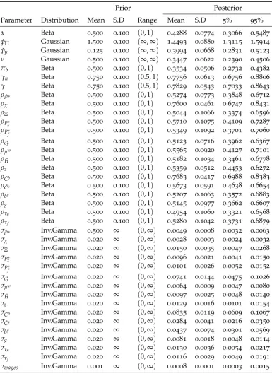
Prior Posterior
Parameter Distribution Mean S.D Range Mean S.D 5% 95%
α Beta 0.500 0.100 (0, 1) 0.4288 0.0774 0.3066 0.5487
φΠ Gaussian 1.500 0.100 (∞,∞) 1.4493 0.0880 1.3115 1.5914
φy Gaussian 0.125 0.100 (∞,∞) 0.3994 0.0668 0.2831 0.5123
ν Gaussian 0.500 0.100 (∞,∞) 0.3447 0.0622 0.2390 0.4506
πb Beta 0.500 0.100 (0, 1) 0.3534 0.0506 0.2732 0.4382
γn Beta 0.750 0.100 (0.5, 1) 0.7756 0.0613 0.6756 0.8806
γ Beta 0.750 0.100 (0.5, 1) 0.7829 0.0543 0.7033 0.8643
ρib∗ Beta 0.500 0.100 (0, 1) 0.5274 0.0773 0.3848 0.6712
ρχ Beta 0.500 0.100 (0, 1) 0.7600 0.0461 0.6747 0.8431
ρΞ Beta 0.500 0.100 (0, 1) 0.5044 0.1066 0.3374 0.6596
ρPx∗ Beta 0.500 0.100 (0, 1) 0.5710 0.1075 0.4109 0.7287
ρP∗f Beta 0.500 0.100 (0, 1) 0.5349 0.1092 0.3701 0.7060
ρc∗x Beta 0.500 0.100 (0, 1) 0.5123 0.0716 0.3962 0.6367
ρµw Beta 0.500 0.100 (0, 1) 0.5565 0.0920 0.4127 0.7101
ρH¯ Beta 0.500 0.100 (0, 1) 0.5182 0.1034 0.3461 0.6778
ρz Beta 0.500 0.100 (0, 1) 0.5359 0.0512 0.4453 0.6272
ρC¯b Beta 0.500 0.100 (0, 1) 0.7683 0.0417 0.6988 0.8383
ρC¯s Beta 0.500 0.100 (0, 1) 0.5673 0.0591 0.4638 0.6654
ρbg Beta 0.500 0.100 (0, 1) 0.5207 0.1063 0.3572 0.6883
ρg Beta 0.500 0.100 (0, 1) 0.5145 0.0977 0.3662 0.6607
ρτn Beta 0.500 0.100 (0, 1) 0.4954 0.1060 0.3321 0.6568
ρτf Beta 0.500 0.100 (0, 1) 0.5280 0.1042 0.3731 0.6879
σib∗ Inv.Gamma 0.500 ∞ (0,∞) 0.0049 0.0008 0.0032 0.0063 σχ Inv.Gamma 0.020 ∞ (0,∞) 0.0028 0.0003 0.0024 0.0032 σΞ Inv.Gamma 0.020 ∞ (0,∞) 0.0150 0.0035 0.0047 0.0268
σP∗
x Inv.Gamma 0.020 ∞ (0,∞) 0.0096 0.0021 0.0041 0.0150
σP∗
f Inv.Gamma 0.020 ∞ (0,∞) 0.0101 0.0026 0.0052 0.0152
σc∗
x Inv.Gamma 0.020 ∞ (0,∞) 0.0741 0.0144 0.0475 0.1026
σµw Inv.Gamma 0.020 ∞ (0,∞) 0.0064 0.0009 0.0047 0.0080
σH¯ Inv.Gamma 0.020 ∞ (0,∞) 0.0097 0.0025 0.0048 0.0140
σz Inv.Gamma 0.020 ∞ (0,∞) 0.0129 0.0016 0.0101 0.0154
σC¯b Inv.Gamma 0.020 ∞ (0,∞) 0.0835 0.0119 0.0609 0.1067
σC¯s Inv.Gamma 0.020 ∞ (0,∞) 0.0284 0.0041 0.0216 0.0350
σbg Inv.Gamma 0.020 ∞ (0,∞) 0.0437 0.0074 0.0301 0.0569
σg Inv.Gamma 0.020 ∞ (0,∞) 0.0081 0.0018 0.0048 0.0114
στn Inv.Gamma 0.020 ∞ (0,∞) 0.0130 0.0036 0.0054 0.0217
στf Inv.Gamma 0.020 ∞ (0,∞) 0.0116 0.0029 0.0049 0.0191
[image:18.595.113.499.86.619.2]4 optimal monetary policy
Given the estimated parameters of the previews section, now we can iden-tify the optimal response from the central bank to credit spreads movements and the benefits within. In order to do this, we follow Bejarano and Charry (2014) and Schmitt-Grohé and Uribe (2004a) were a Welfare function approx-imated up to second order, following Schmitt-Grohé and Uribe (2004b), is maximized over the parameterφωin the Taylor Rule given by equation (56). Then, we compute the welfare loss associated on using the reaction to credit spreads in the benchmark model,φω =0, instead of the one that maximizes the welfare function.
4.1 The Aggregate Welfare Function
Considering the model described in 2th section, Optimal Monetary Policy problem consists in maximizing the following Welfare function overφ∗ω:
φ∗ω =argmax
(
Wt=πbu(cbt; ¯Ctb) +πsu(cst; ¯Cts)
− φ
1+ν
yn,t
zt
1+ωy fΛ t
e
λt
!1+ν ν ∆
t
¯
Htν
+βEtWt+1
(84)
Where
f Λt
1+ν ν =
ψ1ν
πbψ
−1 ν
b λbt
1+ν ν +π
sψ−
1 ν
s λst
1+ν ν
(85)
The welfare function comes from aggregating equation (1) overi. Since we are maximizing the welfare equation approximated to second order, it is not possible to find a reduced form solution. However, it is possible to set a discrete grid forφω and evaluate equation (84) in each grid point, choosing the grid point that gives the highest value. For this exercise we choose grid points with length of0.05.
Additionally, we need to compute welfare loss associated with using an different reaction to credit spreads in the Taylor rule instead ofφ∗ω. To do
this, letWt∗be the welfare level implied byφω∗ andWtathe welfare implied by
any other alternativeφωa 6= φω∗. Welfare loss is measured as the percentage of consumption, Γφ∗a
ω, sacrificed by consumers associated toφ
∗
ω in order to
obtainWta. This implies that
Wt∗[cbt∗,cst∗]≥Wt∗a[(1−Γφ∗a ω)c
b∗
t ,(1−Γφ∗a ω)c
s∗
t ] =Wta (86)
Once the welfare values Wt∗ and Wta are computed, Γφ∗a
ω can be solved
from equation (86).
4.2 The Optimal Response to Credit Spread and Welfare Loss
We compute the optimal response to credit spreadsφ∗ω taking into account all the exogenous shocks in order to reflect all possible disturbances Colom-bian economy can face according to our model. We can see from table 3 that for this caseφω∗ =−0.6. This can be interpreted as the average optimal
Table3: Optimal Response and Welfare Loss on Individual Shocks
Shock φ∗ω 100xΓφω=0.6 100xΓφω=0 S.Dω
ALL -0.60 0% 28.787e-3% 4.2938e-3
χt -2.15 61.581e-3% 102.07e-3% 3.6955e-3
¯
Cbt 0.40 44.202e-3% 6.0920e-3% 1.5930e-3
bgt -4.15 8.2472e-3% 9.5010e-3% 996.22e-6
zt -1.20 3.4382e-3% 12.326e-3% 716.29e-6
¯
Cst -0.80 263.97e-6% 3.9026e-3% 659.36e-6
ibt∗ -1.95 6.3032e-3% 12.070e-3% 635.29e-6
Px,t∗ 6.50 7.4369e-3% 6.3444e-3% 325.95e-6
τf,t -0.15 107.29e-6% 9.7918e-6% 307.69e-6
c∗t -2.40 10.052e-3% 17.438e-3% 285.38e-6
e
Ξt -4.80 698.54e-6% 776.15e-6% 256.20e-6
P∗f,t 5.20 960.42e-6% 779.10e-6% 207.22e-6
gt -1.30 158.77e-6% 505.62e-6% 137.30e-6
¯
Ht -1.10 51.903e-6% 240.42e-6% 112.81e-6
µwt -1.25 24.380e-6% 82.161e-6% 56.939e-6
However, this result is important as it reflects a general recommendation for monetary policy that can be tractable and easy to understand; the same way that it is usually recommended thatφΠ >1 in order to assure inflation stability. For this recommendation to be implementable, we could expect, at least, that the welfare gains associated to this recommendation are higher than those implied byφω =0 for each shock.
Table 3shows the optimal response to credit spreads to each individual shock, as the welfare loss with respect to the recommended reactionφω =
−0.6 and benchmark reactionφω =0. Almost all optimal reaction to credit spreads are negative, except for international prices for imports and exports, and borrowers preference shock. It is immediately clear that for shocks that implyφ∗ω≥0, the economy is better off with the benchmark reactionφω =0,
than with the recommended reactionφω =−0.6, sinceΓφ
ω=0.6 ≥Γφω=0.
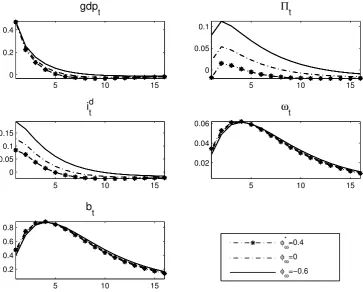
If, for example, we assume a shock to borrowers preferences, ¯Ctb, we can see from the impulse response in figure 1that borrowers are inclined to take more loans from financial intermediaries and, hence, face a higher credit spread. The optimal response for this shock would imply a positive reaction to the increase of the credit spread in order to rise borrowers interest rateibt, so that output and inflation do not fall far from target values. However, the recommended reactionφω =−0.6 would lower borrowers interest rate and increase the deviation of output and inflation from target values, implying a higher deposits interest rate to control these, after all. Finally, we can see that the benchmark reaction φω = 0 falls somewhere in the middle; justifying less welfare loss in this scenario.
We can see, also, from table 3, that the welfare loss from implementing
[image:20.595.177.430.88.305.2]5 10 15 0
0.05 0.1
Π
t5 10 15
0 0.2 0.4
gdp
t
5 10 15
0 0.05 0.1 0.15
i
td5 10 15
0.02 0.04 0.06
ω
t5 10 15
0.2 0.4 0.6 0.8
b
t
φω*=0.4
φω=0
φω=−0.6
Figure1: Impulse Response to shock ¯Ctb using estimated parameters ρC¯tb
and σC¯
tb. Result expressed as percentage points deviations from
steady state.
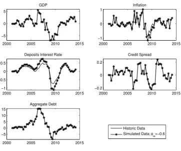
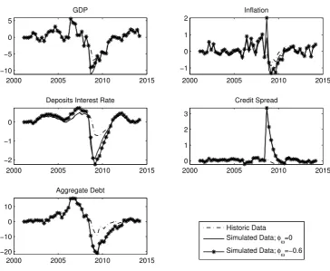
Figure 2shows us that implementing the recommended reaction to credit spreads does not imply significant changes to aggregate variables dynamics. The only simulated variables that show a different dynamic to its historic counterpart are the deposit interest rate and inflation (although it is less pro-nounced).The deposit interest rate shows a positive comovement with the credit spread, which at first glance might seem counterintuitive. As Curdia and Woodford (2010) explains, although the recommended reaction implies a negative reaction to credit spread, it does not mean that the interest rate will actually fall to increases of the credit spread. Near2010credit spreads fell around0.03% below trend, the recommended reaction would imply a rise in the deposit interest rate to discourage a rise of loans; however, this would result in less pressure on price and a lower inflation, which would imply a drop of the deposit interest rate.
So far we have learned that a general recommendation does not imply considerable welfare gains to all shocks compared to the benchmark reaction
[image:21.595.121.485.70.362.2]2000 2005 2010 2015 −5
0 5
GDP
2000 2005 2010 2015
−1 0 1
Inflation
2000 2005 2010 2015
−1 −0.5 0 0.5
Deposits Interest Rate
2000 2005 2010 2015
−0.2 0 0.2
Credit Spread
2000 2005 2010 2015
−5 0 5 10 15
Aggregate Debt
Historic Data
Simulated Data; φω=−0.6
Figure2: Counterfactual analysis between historic data and simulated data assumingφω =−0.6. Result expressed as percentage points devi-ations from trend.
We see from table 3, that must of the optimal reactions are strong com-pared to the recommendedφ∗ω = −0.6; only the optimal reaction to credit
spreads for both types preference shocks and imports taxes shocks are in the(−1, 1)range. However, these differences in the strength of the reaction to the credit spread do not translate to significant welfare loss from setting
φω =0. The biggest welfare loss occurs to the aggregate default probability shock,χt. In this case, household would sacrifice0.102% of their
consump-tion if φω = 0 was set instead of φω∗ = −2.15. A similar logic follows to φω = −0.6, the biggest welfare loss is associated to the aggregate default probability χt, being0.061%. This means that households would sacrifice
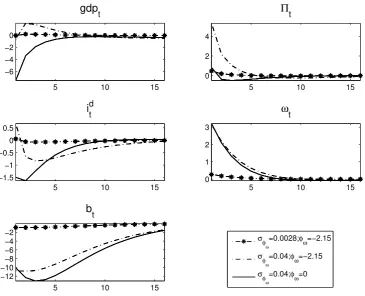
less that0.1% of their consumption from a reaction to spreads ofφω =−0.6, instead ofφ∗ω =−2.15, when an aggregate default probability shock occurs. The reason why most optimal responses to individual shocks are outside the(−1, 1)range can be found in Curdia and Woodford(2010). They found that the strength of the response tends to be grater the lower the persistence of the credit spread is. Curdia and Woodford(2010) found an optimal re-sponse ofφω∗ = −0.66 for the aggregate default probability shock,χt, with
[image:22.595.123.486.63.364.2]5 10 15 −6
−4 −2 0
gdp
t
5 10 15
0 2 4
Π
t5 10 15
−1.5 −1 −0.5 0 0.5
i
td5 10 15
0 1 2 3
ω
t5 10 15
−12 −10 −8 −6 −4 −2
b
t
σφ
ω
=0.0028;φω=−2.15
σφ
ω
=0.04;φω=−2.15
σφ
ω
=0.04;φω=0
Figure3: Impulse Response to shock χt comparing estimated parameters
and Curdia and Woodford’s (2010) σχ. Result expressed as per-centage points deviations from steady state.
Table 3 also provides an interesting fact about this model, the fifth col-umn shows the standard deviation of the credit spread if φω = 0 was as-sumed. There is a positive relation between the standard deviation and the welfare loss compared to both, φω = −0.6 and φω = 0. These standard deviations are not far from the standard deviation of credit spreads implied from historic data on figure 2, which is 1.1384e-3. The sample period se-lected for the estimation was chosen to reflect a monetary policy compatible with the Taylor rule, since for the new millennium Target inflation criteria was adopted, but is not known to have a financial crisis. For times without financial turmoil credit spreads do not tend to be volatile, but periods for with financial stress this spread rises significantly. Chari et al (2008) show evidence of this fact for US economy during the2008financial crisis. They analyzed several measures of credit spreads and showed that these were a stable measure until Lehman Brothers bankruptcy. Specially for the Tbill and Libor rate spread; this measure was a steady measure of0.5%, but the following month after Lehman Brother collapsed it increased up to4.5%.
Figure 3compares the impulse response to a shock to , χt, changing its
standard deviation from0.0028to 0.4 as Curdia and Woodford (2010), but keeping the autoregressive parameter fixed at 0.76. It is clear that credit spreads reacts significantly more in the latter case; as well as the other vari-ables. This figure also compares the optimal reaction to credit spreads to the benchmark. If monetary authority reacted optimally atφω∗ =−2.15 output
[image:23.595.121.487.68.364.2]2000 2005 2010 2015 −10
−5 0 5
GDP
2000 2005 2010 2015
−1 0 1 2
Inflation
2000 2005 2010 2015
−2 −1 0
Deposits Interest Rate
2000 2005 2010 2015
0 1 2 3
Credit Spread
2000 2005 2010 2015
−20 −10 0 10
Aggregate Debt
Historic Data Simulated Data; φω=0 Simulated Data; φω=−0.6
Figure4: Counterfactual analysis between historic data and simulated data assuming σχ = 0.4 in 2008:II. Result expressed as percentage points deviations from trend.
shock, the optimal reaction would imply a significant change to macroeco-nomic variables. Additionally,it also implies an increase in welfare loss. This scenario would imply welfare loss of Γφω=0 = 11.9% andΓφω=0.6 = 7.38%, which are 1,166 and 1,209 times bigger, respectively, compared to the esti-mated standard deviation.
[image:24.595.119.484.62.361.2]5 conclusions
After estimating Bejarano and Charry (2014) model’s structural parameters the optimal response to credit spreads to all disturbances were computed. First, it was analyzed if a general reaction to all disturbances interacting si-multaneously could improve monetary policy with respect to a non respon-sive scenario. Unfortunately, for some disturbances the Colombian economy is better off if the central bank does not react at all. Additionally, this gen-eral response does not imply significant welfare gains, since the impact over macroeconomic variables is null.
Then, each shock was analyzed individually. Similar to Curdia and Wood-ford (2010) the optimal response depended on the source of the disturbance and on its persistence. Although many of these optimal reactions were out-side the (−1, 1) range, similarly to the general recommendation, they did not imply significant welfare gains or responses from output and inflation.
The main explanation to the lack of responsiveness is that the credit spread is not volatile for the sample considered for the estimation. The sample from 2001:I-2014:II is not associated to a financial crisis period, al-though it serves as a good approximation of monetary policy conducted by a Taylor rule, since Inflation targeting was implemented after 2000. How-ever, a counterfactual analysis, that compared the historic data to a simu-lated data where the2008financial crisis spreads to the Colombian economy, showed that after a increase in credit spreads volatility the Colombian econ-omy could obtain considerable gains and stabilized output from reacting to this variable.
references
[1] Bejarano, Jesús., and Charry, Luisa , (2014), "Financial Frictions and Op-timal Monetary Policy in a Small Open Economy",Borradores de Econo-mia,852.
[2] Belke, Ansgar., and Klose, Jens, (2010), "(How) Do the ECB and the Fed React to Financial Market Uncertainty? – The Taylor Rule in Times of Crisis", Ruhr Economic Papers,0166.
[3] Castro, Vítor, (2011), "Can central banks’ monetary policy be described by a linear (augmented) Taylor rule or by a nonlinear rule?",Journal of Financial Stability, Elsevier, vol.7(4), pages228-246.
[4] Chari, V. V., Christiano, Lawrence J., and Kehoe, Patrick J., (2008), "Facts and myths about the financial crisis of2008,"Federal Reserve Bank of MinneapolisWorking Papers666,
[5] Cúrdia, Vasco., and Woodford, Michael , (2009), "Credit frictions and optimal monetary policy", BIS Working Papers, 278, Bank for Interna-tional Settlements.
[6] Curdia, Vasco., and Woodford, Michael , (2010), "Credit Spreads and Monetary Policy", Journal of Money, Credit and Banking, Blackwell Pub-lishing, vol.42(s1), pages3-35.
[7] Gertler, Mark., Gilchrist, Simon., and Natalucci, Fabio M., (2007) "Ex-ternal Constraints on Monetary Policy and the Financial Accelerator,"
[8] González, Andrés., López , Martha., Rodríguez, Norberto., and Téllez, Santiago , (2013), "Fiscal Policy in a Small Open Economy with Oil Sector and non-Ricardian Agents," Borradores de Economia,759, Banco de la Republica de Colombia.
[9] Hamann, Franz., Pérez, Julián., and Rodríguez , Diego , (2006), "Bring-ing a DSGE model into policy environment in Colombia". Banco de la República.
[10] Huang, Yu-Fan, (2015), "Time variation in U.S. monetary policy and credit spreads",Journal of Macroeconomics,Elsevier, vol.43(C), pages205
-215.
[11] López, Martha., Prada ,Juan David., and Rodríguez, Norberto , (2009), "Evidence for a Financial Accelerator in a Small Open Economy,and Im-plications for Monetary Policy,"Ensayos Sobre Política Económica, Banco de la República - ESPE, vol.27(60), pages12-45, December.
[12] Martin, Christopher.. and MILAS , Costas, (2013), " Financial crises and monetary policy: Evidence from the UK", Journal of Financial Stability
,9(4),654–661.
[13] Mishkin, Frederic S, (2008), "Monetary policy flexibility, risk manage-ment, and financial disruptions : a speech at the Federal Reserve Bank of New York, New York", Speech 353, Board of Governors of the Fed-eral Reserve System (U.S.).
[14] Prada , Juan David., Rojas ,Luis Eduardo (2009), "La elasticidad de Frisch y la transmisión de la política monetaria en Colombia," Bor-radores de Economia,555, Banco de la Republica de Colombia.
[15] Pfeifer., Johannes, (2014) "A Guide to Specifying Observation Equations for the Estimation of DSGE Models" University of Mannheim
[16] Schmitt-Grohe, Stephanie., and Uribe, Martin, (2003), "Closing small open economy models,"Journal of International Economics, Elsevier, vol.
61(1), pages163-185, October.
[17] Schmitt-Grohe,Stephanie ., and Uribe, Martin , (2004a), "Optimal Oper-ational Monetary Policy in the Christiano-Eichenbaum-Evans Model of the U.S. Business Cycle",NBER Working Papers,10724, National Bureau of Economic Research, Inc.
[18] Schmitt-Grohe,Stephanie ., and Uribe, Martin , (2004b), "Solving dy-namic general equilibrium models using a second-order approxima-tion to the policy funcapproxima-tion", Journal of Economic Dynamics and Control, Elsevier, vol.28(4), pages755-775.
[19] Stock , James H,.and Watson, Mark W. ,(1999) "Forecasting Inflation,"
NBER Working Papers, 7023, National Bureau of Economic Research, Inc.
[20] Taylor, John B., (2008) , " “Monetary Policy and the State of the Econ-omy: Testimony before the Committee on Financial Services" , U.S. House of Representatives, February26,2008.