Color Image Segmentation Using Multispectral Random Field Texture
Model & Color Content Features
Orlando J. Hernandez
E-mail: hernande@tcnj.edu
Department Electrical & Computer Engineering, The College of New Jersey
Ewing, New Jersey 08628-0718, USA
and
Alireza Khotanzad
E-mail: kha@engr.smu.edu
Department of Electrical Engineering, Southern Methodist University
Dallas, Texas 75275-0338, USA
ABSTRACT
This paper describes a color texture-based image segmentation system. The color texture information is obtained via modeling with the Multispectral Simultaneous Auto Regressive (MSAR) random field model. The general color content characterized by ratios of sample color means is also used. The image is segmented into regions of uniform color texture using an unsupervised histogram clustering approach that utilizes the combination of MSAR and color features. The performance of the system is tested on two databases containing synthetic mosaics of natural textures and natural scenes, respectively.
Keywords: Color Texture, Multispectral Random Field Models, Color Texture Segmentation
1. INTRODUCTION
This paper describes a color texture-based segmentation system. The approach involves characterizing color texture using features derived from a class of multispectral random field models and color space. These features are then used in an unsupervised histogram clustering-based segmentation algorithm to find regions of uniform texture in the query image.
Texture information has been used in the past for the characterization of imagery, however the previously proposed approaches have either considered only gray level textures or pixels based color content and not color texture [1]. The utilized segmentation algorithm in some approaches has also not been completely unsupervised [2]. The contributions of this paper are as follows:
• Texture characterization by a mix of multispectral random field based features and color content features.
• Development of a completely unsupervised color-texture-based segmentation algorithm and demonstration of its effectiveness.
• Demonstration of the effectiveness of the proposed approach on two databases containing 1) synthetic mosaics of natural textures and 2) natural scenes.
Related Studies
The main aspect to this work is segmentation of color texture images. Accordingly, some salient previous studies related to this topic are reviewed in this section.
The texture segmentation algorithm in [3] considers features extracted with a 2-D moving average (MA) approach. The 2-D MA model represents a texture as an output of a 2-D finite impulse response (FIR) filter with simple input process. The 2-D MA model is used for modeling both isotropic and anisotropic textures. The maximum likelihood (ML) estimator of the 2-D MA
model is used as texture features. Supervised and unsupervised texture segmentation are considered. The texture features extracted by the 2-D MA modeling approach from sliding windows are classified with a neural network for supervised segmentation, and are clustered by a fuzzy clustering algorithm for unsupervised texture segmentation.
Mirmehdi and Petrou in [4] present an approach to perceptual segmentation of color image textures. Initial segmentation is achieved by applying a clustering algorithm to the image at the coarsest level of smoothing. The image pixels representing the core clusters are used to form 3D color histograms that are then used for probabilistic assignment of all other pixels to the core clusters to form larger clusters and categorize the rest of the image. The process of setting up color histograms and probabilistic reassignment of the pixels to the clusters is then propagated through finer levels of smoothing until a full segmentation is achieved at the highest level of resolution.
Deng and Manjunath [1] also present a new method (JSEG) for unsupervised segmentation of color-texture regions in images. It consists of two independent steps: color quantization and spatial segmentation. In the first step, colors in the image are quantized to several representative classes that can be used to differentiate regions in the image. Applying the criterion to local windows in the class-map results in the “J-image,” in which high and low values corresponded to possible boundaries and interiors of color-texture regions. A region growing method is then used to segment the images based on the multiscale J-images. This method is still pixel based, and we contrast results of image segmentation of this algorithm with our approach later in this paper.
2. COLOR TEXTURE CHARACTERIZATION WITH MULTISPECTRAL SIMULTANEOUS AUTOREGRESSIVE MODEL
In this work, the texture of the color images is characterized using a class of multispectral random field image model called the Multispectral Simultaneous Autoregressive (MSAR) model [5], [6]. The MSAR model has been shown to be effective for color texture synthesis and classification [5], [6]. For mathematical simplicity, the model is formulated using a toroidal lattice assumption. A location within a two-dimensional M x M lattice is denoted by s = (i, j), with i, j being integers from the set J = {0, 1, …, M-1}. The set of all lattice locations is defined as Ω = {s = (i, j) : i, j ∈ J}. The value of an image observation at location s is denoted by the vector value
neighboring pixels, both within and between image planes, according to the following model equation:
∑ ∑
= ∈ = ρ + ⊕ θ = P 1 j N i i i ij i ij P 1 i ), ( w ) ( y ) ( ) ( y r s r s r s K (1) where:yi(s) = Pixel value at location s of the ith plane s and r = two dimensional lattices
P = number of image planes (for color images, P = 3, representing: Red, Green, and Blue planes)
Nij = neighbor set relating pixels in plane i to
neighbors in plane j (only interplane neighbor sets, i.e. Nij, i ≠ j, may include the (0,0) neighbor)
θij = coefficients which define the dependence of yi(s)
on the pixels in its neighbor set Nij
ρi = noise variance of image plane i
wi(s) = i.i.d. random variables with zero mean and
unit variance
⊕ denotes modulo M addition in each index
The parameters associated with the MSAR model are θ and ρ vectors which collectively characterize the spatial interaction between neighboring pixels within and between color planes. These vectors are taken as the feature set fT representing the underlying color texture of
the image.
A least squares (LS) estimate of the MSAR model parameters is obtained by equating the observed pixel values of an image to the expected value of the model equations [5]. This leads to the following estimates:
⎥
⎦
⎤
⎢
⎣
⎡
⎥
⎦
⎤
⎢
⎣
⎡
=
∑
∑
∈ −∈Ω s Ω
s
s
s
q
s
q
s
q
(
)
(
)
(
)
y
(
)
θ
ˆ
i i 1 T i i i (2) and(
)
∑
∈−
=
ρ
Ω ss
q
θ
s
iT i 2i 2
i
y
(
)
ˆ
(
)
M
1
ˆ
(3)
where:
[
T]
TiP T 2 i T 1 i
i
θ
θ
θ
θ
=
L
(4)
[
T]
TiP T 2 i T 1 i
i
(
s
)
y
(
s
)
y
(
s
)
y
(
s
)
q
=
L
(5)
{
j ij}
ij
(
s
)
=
col
y
(
s
⊕
r
)
:
r
∈
N
y
(6)
This model has been shown to be effective for color texture synthesis as well in [6], and the resulting synthetic images can be visually compared to the original images, and observed to be very similar in appearance to the images from which the models were derived.
3. COLOR CONTENT CHARACTERIZATION
In addition to modeling color texture, the general color content of the image is also important. Additional features focusing on the color alone are also considered. This is done using the sample mean of the pixel values in the red, green, and blue (RGB) planes. The defined feature vector is:
⎪⎭
⎪
⎬
⎫
⎪⎩
⎪
⎨
⎧
µ
µ
µ
µ
=
b r g rC
,
)
)
)
)
f
(7)
with
µ
ˆ
is being the sample mean of the respective color component. The reason for using these specific ratios, instead of some of the other ratios formed by the other combinations of the color means, is that this same relationship was used to form ratios of the ρ parameters of the MSAR model used for texture classification in [5] with very positive results. Also, the reason for using ratio of color means instead of color means themselves is that such a ratio is illumination invariant. Assuming that the observed value at each pixel is a product of illumination and spectral reflectance, the ratios of the color means are invariant to uniform changes in illumination intensity (i.e. the power of the illumination source changes uniformly across the spectrum). This kind of uniform change would cause eachµ
ˆ
i to change by the same scale factor making the defined ratios invariant to illumination changes. This property makes the color-content features more robust. In the event that the denominator of any of the ratios of the color means goes to zero, the color mean with a value of zero is changed to a value of one to avoid the mathematical exception of dividing by zero. This case; however, is very unlikely, since we are dealing with textures and natural images that do not tend to have large areas (i.e. the feature extraction sliding window to be described later) with a solid color extreme.The combination of fC and fT features is used to represent
a color texture region in this work. These features are collectively referred to as Color Content, Color Texture (C3T) features.
4. UNSUPERVISED IMAGE SEGMENTATION WITH A HISTOGRAM-BASED CLUSTERING ALGORITHM
The segmentation algorithm used in this work relies on scanning the image with a sliding window and extracting C3T features from each window. These features are then clustered using an unsupervised histogram-based algorithm. Mapping the identified clusters back into the image domain results in the desired segmentation.
Feature Extraction with a Sliding Window
of 4 pixels. The best W is found automatically as described in later sections.
M
W
W
M
[image:3.595.76.286.105.297.2]D
Fig. 1. Feature vector extraction with a sliding window
As the window size is increased, the overlap between areas covered by adjacent windows increases, since D is constant, and thus the redundancy of information from feature vectors obtained from larger adjacent windows increases as W increases. It was decided not to increase D for the larger W values, and thus not to reduce the spatially adjacent vectors redundancy, because as W increases the likelihood of capturing a more heterogeneous image area increases as well. Leaving redundancy between adjacent vectors helps the cohesion and convergence of the clustering process, from a spatial perspective.
The texture bounded by each window is characterized using the C3T features. The neighborhood used for the MSAR model is a set that contains neighbors above, below, to the left, and to the right of the pixel as illustrated in Fig. 2. The same neighbor set is used for both inter and intra-planes of the model.
X
X O X
X
Fig. 2. Neighbor set used with the MSAR model
This neighbor set results in a 20-dimensional fT. Therefore
together with the two-dimensional color content feature set, a 22-dimensional C3T feature vector, f, is used to characterize each window.
Clustering Algorithm
Once all 22-dimensional f features are extracted from the sliding window, they are clustered in the feature space using an unsupervised histogram-based peak climbing algorithm [7], [8]. The 22-dimensional histogram is generated by quantizing each dimension according to the following:
( )
( )
( )
;
k
1
,
2
,
,
N
Q
k
f
k
f
k
CS
=
max−
min=
K
(8)
( )
( )
( )
1
;
k
1
,
2
,
,
N
k
CS
k
f
k
f
INT
d
mink
=
K
⎭
⎬
⎫
⎩
⎨
⎧
+
−
=
(9)
where:
N = total number of features (22 in this case) CS(k) = length of the kth side of histogram cell fmax(k) = maximum value of the kth C3T features
fmin(k) = minimum value of the kth C3T features
Q = total number of quantization levels dk = kth index for a histogram cell
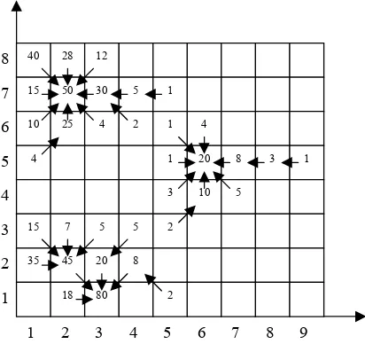
Since the dynamic range of the vectors in each dimension can be quite different, the cell size for each dimension would be different. Hence the cells will be hyperboxes. Next, the number of feature vectors falling in each hyperbox is counted and this count is associated with the respective hyperbox creating the required histogram. After the histogram is generated in the feature space, a peak climbing clustering approach is utilized to group the features into distinct clusters. This is done by locating the peaks of the histogram. In Fig. 3 this peak climbing approach is illustrated for a two-dimensional space example.
40 28 12
15 50 30 5 1
10 25 4 2 1 4
4 1 20 8 3 1
3 10 5
15 7 5 5 2
35 45 20 8
18 80 2
1 2 3 4 5 6 7 8 9
1 2 3 4 5 6 7 8
Fig. 3. Illustration of the Peak Climbing approach for a two-dimensional feature space example
[image:3.595.317.523.396.590.2]features grouped in the same cluster are tagged as belonging to the same category.
A major component of this algorithm is the number of quantization levels associated with each dimension. To decide this parameter, the total number of non-empty cells and the percentage of them capturing only one vector for each selection of quantization levels are examined. The best number of quantization levels is selected as the largest one that maximizes the measure below [16].
(
ci ui)
uii
N
N
N
M
=
−
×
(10)
where:
Nci = number of non-empty cells
Nui = number of cells capturing only one sample
The algorithm also includes a spatial domain cluster validation step. This step involves constructing a matrix B for each cluster m as:
otherwise
0
)
j
,
i
(
B
m
cluster
sample
if
1
)
j
,
i
(
B
m m
=
∈
=
(11)
The (i, j) index corresponds to the location of a sliding window. A cluster is considered compact if only a very small number of its 1-elements have a 0-element neighbor, i.e. a cluster is considered valid (compact) if only a very small number of its elements have neighboring elements that do not belong to that cluster. A cluster that does not pass this test is merged with a valid cluster that has the closest centroid to it.
During the segmentation process, the best window size for scanning the image is chosen in an unsupervised fashion. The optimum window size is obtained by sweeping the image with varying window sizes (4 to 28 pixels in steps of 4 pixels), and choosing the smallest one out of at least two consecutive window sizes that produce the same number of clusters.
5. RESULTS
The performance of the system on two different databases is reported in this section.
Test Databases
Two databases are used to test the performance of the proposed approach. These databases are referred to as Natural Texture Mosaics Database, and Natural Scenes Database.
Natural Textures Mosaics Database: The Natural Texture Mosaics Database is a collection of images that are mosaics of natural textures constructed from texture images available in [9]. This collection includes 200 128 x 128 images with mosaics put together at random in terms of the arrangement and the type of the texture regions used. This database is constructed to measure and investigate the effectiveness of the algorithm in a controlled environment.
Natural Scenes Database: The Natural Scenes Database is a collection of images, which is comprised of natural scenes available in [10]. This collection has 400 images of various sizes that include 120 x 80, 80 x 120,
128 x 85, and 85 x 128 pixels. This database was constructed to test the performance on real imagery.
Segmentation Results
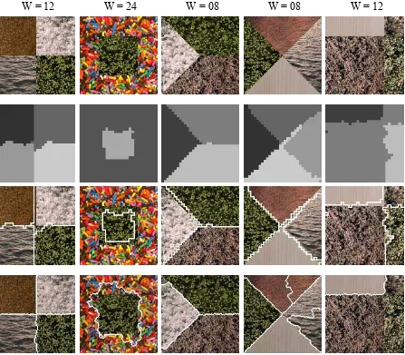
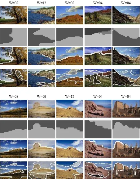
The performance of the proposed segmentation algorithm and the associated features is illustrated in Figs. 4 and 5. Fig. 4 shows five images each containing a number of different textures. These image mosaics are created from texture samples available in [9]. Below each image the segmentation result is presented in the form of a gray-level image with pixels belonging to the same texture having the same gray level. In the next row, the boundaries of the segmented regions are shown as superimposed white lines. At the top of the figures, the size of the optimal window found by the algorithm is shown. Fig. 5 shows the segmentation results for several natural scene images. These natural scene images are available in [10]. It is observed that the proposed algorithm performs quite well and is capable of localizing uniform color textures in each image.
In Fig. 4 and Fig. 5, we also compare the results of our approach with the image segmentation results achieved using the JSEG method described in [1]. The JSEG results were obtained from applying the images to the programs made available by the JSEG authors at the Internet site http://maya.ece.ucsb.edu/JSEG/. The obtained region boundaries are superimposed on the original images. The JSEG results are displayed in the last rows of Figs. 4 and 5. It can be seen that our segmentation results have a better match with perceptual boundaries in the images. The JSEG method over segments most of the natural scene images and misses or mislabels some boundaries in mosaic images. However; the approach proposed in this work is 3 to 5 times more computationally intensive than the JSEG method, e.g. it takes about 15 seconds to segment a 128 x 128 pixels image with this method on a Pentium II 400MHz processor versus about 5 seconds with the JSEG method.
6. CONCLUSIONS
In this work, a novel color texture-based approach to image segmentation is developed. Features derived from the Multispectral Autoregressive (MSAR) random field model with a 4-neighbor set, and the RGB color space represented by the ratios of the true color plane means are used to characterize the color texture content of the image. These features are extracted from the image using a sampling window that slides over the entire image, and are used in conjunction with an unsupervised clustering-based segmentation algorithm to segment the images into regions of uniform color texture. The image regions are obtained by mapping back to the spatial domain of the image the significant clusters obtained in the 22-dimensional feature space during the clustering process. The effectiveness of the approach has been demonstrated using two different databases containing synthetic mosaics of natural textures and natural scenes. Furthermore, applications of this new perceptually compatible image segmentation method are possible in the areas of video processing and event detection, and video database and retrieval systems.
7. REFERENCES
[2] J. R. Smith and S-F. Chang, Integrated Spatial and Feature Image Query, Multimedia Systems – ACM - © Springer-Verlag 1999, vol. 7, no. 2, 1999, pp. 129-140. [3] K. B. Eom, Segmentation of monochrome and color textures using moving average modeling approach, Elsevier Science B. V. Image and Vision Computing, no. 17, 1999, pp. 233-244.
[4] M. Mirmehdi and M. Petrou, Segmentation of Color Textures, IEEE Trans. on Pattern Analysis and Machine Intelligence, vol. 22, no. 2, 2000, pp. 142-159.
[5] J. W. Bennett, Modeling and Analysis of Gray Tone, Color, and Multispectral Texture Images by Random Field Models and Their Generalizations, Ph.D. Dissertation, Southern Methodist University, 1997.
[6] J. W. Bennett and A. Khotanzad, Multispectral Random Field Models for Synthesis and Analysis of Color
Images, IEEE Trans. on Pattern Analysis and Machine Intelligence, vol. 20, no. 3, 1998, pp. 327-332.
[7] A. Khotanzad and J. Y. Chen, Unsupervised Segmentation of Textured Images by Edge Detection in Multidimensional Features, IEEE Trans. on Pattern Analysis and Machine Intelligence, vol. 11, no. 4, 1989, pp. 414-421.
[8] A. Khotanzad and A. Bouarfa, Image Segmentation by a Parallel, Non-Parametric Histogram Based Clustering Algorithm, Pattern Recognition, vol. 23, no. 9, 1990, pp. 961-963.
[9] Vision and Modeling Group, MIT Media Laboratory, Vision Texture (VisTex) database, http://www-white.media.mit.edu/vismod/, 1995.
[image:5.595.75.522.252.643.2][10]Corel Corporation, Professional Photos CD-ROM Sampler – SERIES 200000, 1994.
Fig. 4. Segmentation results for four natural texture mosaic images, 1st row: Original image, 2nd row: Segmentation results, 3rd row: Texture boundaries corresponding to segmentation results, 4th row: Segmentation using JSEG method
Fig. 5. Segmentation results for eight natural scene images, 1st row: Original image, 2nd row: Segmentation results, 3rd row: Texture boundaries corresponding to segmentation results, 4th row: Segmentation using JSEG method