Interpolation of paleoclimatology datasets

(1)

Interpolation of paleoclimatology datasets

Luis E. NIETO-BARAJAS

Departamento de Estadística, Instituto Tecnológico Autónomo de México (ITAM), Río Hondo 1, Col. Progreso Tizapán, 01080 CDMX, México

Email: lnieto@itam.mx

Received: February 17, 2017; accepted: January 22, 2018

RESUMEN

Los datos de paleoclima incluyen mediciones de la cantidad de dióxido de carbono en la atmosfera, así como el nivel y temperatura de los océanos, entre otras. Los registros recientes de datos de cambio climático se han realizado en tiempos equidistantes, es decir, las distintas variables se han medido al mismo tiempo para que puedan llevarse a cabo estudios de asociación. Sin embargo, no hay registros de datos de hace miles de millones de años. Los científicos han tenido que diseñar formas alternativas de obtener esta información, por lo general a través de mediciones indirectas como las basadas en núcleos de hielo, donde tanto la variable de interés como el tiempo de medición tienen que estimarse. Como resultado de estos procedimientos, los datos de paleoclima son una colección de observaciones que no están distribuidas de manera uniforme. Aquí revisamos un método estadístico bayesiano para producir series equiespaciadas y lo aplicamos a tres bases de datos de paleoclima que van de 300 millones de años atrás a la fecha.

ABSTRACT

Paleoclimatology data includes measures of the amount of carbon dioxide in the atmosphere and level and temperature of the oceans, among others. Recent records of climate change data were done at equidistant times; the different variables were typically measured at the same time to allow for association studies among them. However, there are no registered records of climate change data for thousands or millions of years ago. Scientists have had to device alternative ways of measuring these quantities. These methods are usually a result of indirect measurements, such as ice coring, where both the variable of interest and the time have to be estimated. As a result, paleoclimate data are a collection of time series where observations are unequally spaced. Here we review a Bayesian statistical method to produce equally spaced series and apply it to three paleoclimatology datasets that span from 300 million years ago to the present.

Keywords: Bayesian analysis, EPICA, Gaussian process, interpolation, pliocene, paleozoic.

1. Introduction

Direct and continuous measurements of carbon di-oxide (CO2) in the atmosphere extend back only to the 1950s (British Antarctic Survey, 2014). However, scientists developed alternative ways of measuring greenhouse gases (GHG) concentrations in the earth’s atmosphere that prevailed far in the past. One of these techniques is based on ice core sampling. The core samples are cylinders of ice drilled out of an

(2)

model (Loulergue et al., 2007) to further compensate for differences in the age of the gas and the age of the surrounding ice.

The European Project for Ice Coring in Antarctica (EPICA) drilled two deep ice cores at Kohnen and Concordia. At the latter station, also called Dome C, the team of researchers produced climate records focusing on water isotopes, aerosol species and GHG. Tempera-ture measurements are not observed but inferred from deuterium observations (Jouzel et al., 2007).

To estimate GHG concentrations in the earth beyond one million years ago, other techniques are required. Recently, Montanez-Boti et al. (2015) esti-mated CO2 levels from the Pliocene period (around three million years ago). These estimations were based on the boron isotopic composition of Globigeri-noides ruber, a surface mixed-layer dwelling planktic foraminiferal species from the Ocean Drilling Pro-gram (ODP) site 999. The boron isotopic composition is a well-constrained function of seawater pH. It is well correlated with the aqueous concentration of CO2 (CO2aq). In the absence of major changes in

surface hydrography, CO2aq is largely a function of

atmospheric CO2 levels.

On the other hand, for the late Paleozoic degla-ciation (around 300 million years ago), Montanez et al. (2007) use the stable isotopic compositions of soil-formed minerals, fossil- plant matter, and shallow-water brachiopods to estimate atmospheric partial pressure of carbon dioxide (pCO2) and tropical marine surface temperatures.

The aim of this paper is to interpolate several paleoclimate datasets and make them available to the global community for further statistical analysis.

There are several interpolation methods for climate time series, which are mostly summarized in Mudelsee (2010). The most popular stochastic interpolation method is linear interpolation, which assumes a standard Brownian motion process (e.g., Chang, 2012; Eckner, 2012). More recently, Nie-to-Barajas and Sinha (2015) proposed an interpola-tion method based on a Gaussian process model with a novel parameterization of the variance function. They compared their proposal with alternative mod-els and showed that it is superior according to some specific fitting measures.

Interpolation of climate time series has been criti-cized by several authors (e.g., Schulz and Stattegger,

1997; Schulz and Mudelsee, 2002) arguing a loss of high-frequency variability and a spectral bias towards low frequencies. However, Bayesian stochastic in-terpolation methods account for the uncertainty in the estimation by means of the posterior predictive distribution, which allows to produce not only point predictions but posterior credible intervals for the interpolated series.

According to Rehfeld and Kurths (2014), paleo-climate time series are more challenging than the data in other disciplines since neither observation time nor the climatic variable are known precisely. Both have to be reconstructed, resulting in irregular and age-uncertain time series. To avoid interpola-tion these authors have studied the performance of dependence measures such as the Gaussian kernel based cross correlation and a generalized mutual information function. On the other hand, individual time series models have been proposed to account for the uneven time spacing. Robinson (1977) and Schulz and Mudelsee (2002) defined a first order autoregres-sive process where the autocorrelation parameter as well as the variance of the errors are functions of the time difference between two observed points. Alter-natively, Polanco-Martínez and Faria (2015) estimate the wavelet spectrum of the time series.

The contents of the rest of the paper are as follows: In Section 2 we first present the datasets to interpo-late. In Section 3 we recall the Bayesian thinking and describe the Gaussian process Bayesian model used for interpolation in Section 4. The actual interpolation of the series is presented in Section 5 and we conclude with some final remarks in Section 6.

2. Datasets

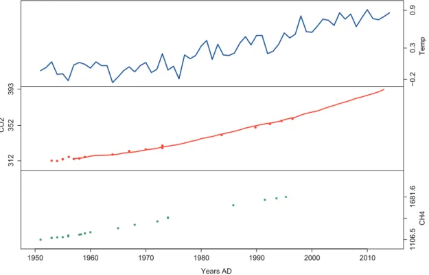
We will be using several datasets with different time scales. Variables measured are temperature, CO2 and methane (CH4). Actual temperatures are not usually provided. Instead, temperature anomalies with re-spect to a specific reference value are reported. The scale used is degrees centigrade (ºC). CO2 is usually reported in parts per million by volume (ppmv) and CH4 is measured in parts per billion by volume (ppbv). We start with the most recent information and progress backwards in time to approximately 300 million years ago.

(3)

The top panel contains global land temperature anomalies with respect to the mean temperature in the years 1951-1980 (Hansen et al., 2010). The middle panel contains CO2 values from two different sources: atmospheric values derived from flask air samples collected at the South Pole (line) (Keeling et al., 2008), and Law Dome ice core records (dots) (MacFarling Meure et al., 2006). As can be seen, the dots follow the trend of the line, which confirms the ice core sample acts as an accurate measure of atmospheric gas concentrations. The bottom panel contains methane records from the law dome ice core (MacFarling Meure et al., 2006).

The second dataset covers the marine isotope stage, including a long range of 800 000 years before present. These data are shown in Figure 2. The top panel presents temperature anomalies with respect to the average temperature of the millennium (Jou-zel et al., 2007). The middle panel includes carbon dioxide concentrations (Luthi et al., 2008), and the bottom panel contains methane values (Loulergue et al., 2008).

The third dataset covers the late Pliocene extend-ing from 2.3 to 3.3 million years ago. The data are shown in Figure 3. The top panel contains interpo-lated relative mean annual sea surface temperature (SST) change (Montanez-Boti et al., 2015). The second panel presents the interpolated relative mean annual surface air temperature change (van de Wal et al., 2011). The bottom panel shows atmospheric CO2 reconstructions based on multi-site boron-isotope records (Montanez-Boti et al., 2015).

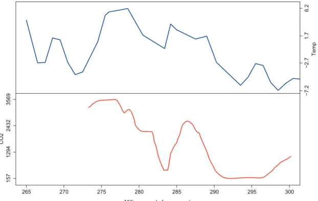
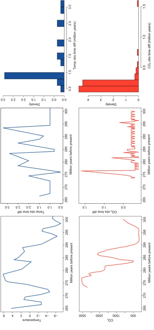
The fourth dataset covers the late Paleozoic de-glaciation from 265 to 300 million years ago. The data are presented in Figure 4. The top panel shows paleotropical SSTs and the bottom panel presents estimated atmospheric pCO2. Both datasets were obtained from Montanez et al. (2007).

3. Bayesian thinking

Bayesian statistics is an alternative way of making inference about the unknown parameters in a prob-ability model. It is based on decision theory, which establishes the foundations of inferential procedures

1950 1960 1970 1980 1990 2000 2010 1106.5

1681.6

CH

4

312

352

393

CO

2

−0.2

0.

30

.9

Years AD

Temp

(4)

0 200 400 600 800

34

26

24

90

7

CH

4

172

235

299

CO

2

−10.

6−

2.

65

.5

Thousand years before present

Te

mp

Fig. 2. EPICA dome C ice core 800 thousand years data. Top: Antarctic temperature anomalies; middle: CO2; bottom: CH4.

2.4 2.6 2.8 3.0 3.2

23

43

45

2

CO

2

−3.6

−0.7

2.

3

−0.9

1.

13

.2

Million years before present

Temp

A

Temp

S

(5)

by treating them as decision problems (DeGroot, 2004). As part of the inferential process, it is neces-sary to quantify the uncertainty about the unknown quantities (parameters or future observations) by using probability distributions. This quantification can reflect the beliefs of the statistician, or the lack of knowledge about the problem. As a consequence of this quantification, all observable variables, as well as the fixed parameters of the model, are described through probability distributions, simplifying so the inferential procedure. For a comprehensive exposi-tion on the Bayesian foundaexposi-tions see Bernardo and Smith (2000) and references therein.

The methodology establishes how to formally combine an initial (prior) degree of belief of a re-searcher with currently measured or observed data in such a way that it updates the initial degree of belief. The result is called posterior belief. This process is called Bayesian inference since the updating pro-cess is carried out through the application of Bayes’ theorem. The posterior belief is proportional to the product of the two types of information, the prior information about the parameters in the model, and the information provided by the data. This second

part is usually thought of as the objective portion of the posterior belief. We explain this process below. In what follows we denote by f (•) a density function of the argument inside the parenthesis, and a vertical bar “|” to denote conditional probabilities.

Let X = (X1, X2,..., Xn) be a set of random variables

whose joint distribution is denoted by f (x|θ), where θ is a parameter vector that characterizes the form of the density. In the case of independence, f (x|θ) =

(xi|θ) f Πn

i=1 where the marginal distribution for each of the Xi is coming from a probability model with

density function f (xi|θ). Function f (x|θ) is usually

referred to as the likelihood function. Prior available information on the parameter is described through a prior distribution f(θ) that must be specified or mod-eled by the researcher. Then formally, it follows that

f (θ|x) = f (x_f|θ₍_x) ₎f (θ) (1)

where f(x) is the marginal joint density of x defined as f(x) = ∫f (x|θ) f (θ)dθ if θ is continuous, and f(x) = ∑θf (x|θ)f(θ) if θ is discrete. This is Bayes’ theorem

that rules the updating of the information. Consider-ing that f(x) is just a constant for θ, then the updating

15

71

294

2432

3569

CO

2

−7.2

−2.7

1.

76

.2

Temp

265 270 275 280 285 290 295 300

(6)

mechanism can be simply written as f(θ|x) ∝f(x|θ) f(θ), where “∝” indicates proportionality. In other

words, the posterior distribution of the parameters, conditional on the observed data, is proportional to the product of the likelihood function and the prior degree of belief. Any inference on the parameters is now carried out using the posterior distribution f(θ|x).

As can be proved (DeGroot, 2004), the only criterion for optimal decision making, consistent with the axiomatic system, is the maximization of the expected utility. Alternatively, this criterion is equivalently replaced by the minimization of a loss function. Therefore, in the Bayesian framework, parameter estimation is done by minimizing the ex-pected value of a specified loss function l(θ̂ , θ) with respect to θ̂, where the expected value is taken with respect to the posterior distribution of the parameter θ given the data y. In particular, a quadratic loss function l(θ̂ , θ) = (θ̂ – θ)2_{leads to the posterior mean} θ̂ = E(θ|x) as an optimal estimate for the parameter. On the other hand, a linear loss function l(θ̂ , θ) = |θ̂ – θ|yields the median of the posterior distribution as an optimal estimate θ̂ for θ.

When the main purpose of modeling is prediction, then the observed data x are used to predict future observations XF by means of the posterior predictive

distribution. In the continuous case the predictive distribution is defined as

f (xF|x) = ∫ f (xF|θ, x) f (θ|x)dθ (2)

where f (xF| θ, x) becomes f (xF|θ) in the case that XF

and X are conditionally independent given the param-eter θ. In (2) the parameters have been marginalized (integrated out). Therefore, only information in the observed data is used in the prediction. Finally, the optimal point predictor x̂ F, assuming a quadratic loss

function, is the mean of the predictive distribution, i.e. E(XF|x).

For the interested reader, we suggest Renard et al. (2006), who provide an excellent review of the Bayesian thinking applied to environmental statistics.

4. A Gaussian process model for interpolation

The model of Nieto-Barajas and Sinha (2015) aims to produce equally spaced observations via stochas-tic interpolation. It assumes a Gaussian process with a correlation function parameterized in terms

of a parametric survival function and allows for positive or negative correlations. For parameter estimation they follow a Bayesian approach. Once posterior inference on the model parameters is done, interpolation is carried out by using the pos-terior predictive conditional distributions of a new location given a subset of size m of neighbors, in a sliding windows manner. The number of neighbors m is decided by the user. This procedure is similar to what is done in spatial data known as Bayesian kriging (e.g. Handcook and Stein, 1993; Bayraktar and Turalioglu, 2005).

4.1 Model

In time series analysis, the observed data are a result of an evolving process in time where independence in the observations is no longer hold. The probability law that generates the data is typically described in terms of a stochastic process which characterizes all dependencies among the observations. A stochastic process can be thought of as a family of random variables linked via a parameter (usually time) which takes values on a specific domain (usually the real numbers).

Let {Xt} be a continuous time stochastic process

defined for an index set t ∈ T⊂R and which takes

values in a state space χ ⊂R. We will say that Xt₁,

Xt₂..., X_tn is a sample path of the process at possible

unequal times t1,t2,...,tn with n > 0. In a time series

analysis we only observe a single path that is used to make inference about the model. This is possible since the likelihood is defined as the joint distribu-tion of the observed path, which depends on the n observed times. This will later be given in (5) for our particular model.

It is assumed that Xt follows a Gaussian process

with constant mean E(Xt) = µ and covariance function

Cov(Xs, Xt) = Ʃ(s, t). In notation

Xt ~ GP (µ,Ʃ(s, t)), (3)

this assumption implies that the joint distribution of the path (Xt₁, Xt₁..., X_tn) is a multivariate normal with

mean vector (µ,...,µ) of dimension n, and variance-co-variance matrix of dimension n × n with (i, j)th element Ʃ(ti, tj).

(7)

In this case it is said that the covariance function is isotropic (Rasmussen and Williams, 2006). By assuming a constant marginal variance for each Xt,

the covariance function can be expressed in terms of the correlation function R(s,t) as Ʃ(s,t) = s2_R₍_s_,_t_). Nieto-Barajas and Sinha (2015) noted that isotropic correlation functions behave like survival functions as a function of the absolute time difference |t – s|. In particular, they considered two alternatives: A Weibull survival function Sθ(t) = exp(–λtα), and a

log-logistic survival function Sθ(t) = (1 + λtα)–1, with

θ= (λ, α) in either case. Therefore, the covariance function they proposed is

Ʃσ2,θ,β (s, t) = σ2Sθ (|t – s|)(–1)β|t–s| (4) with β ∈ {1, 2} in such a way that β = 1 implies a

negative/positive correlation for odd/even time dif-ferences |t – s|, and it is always positive regardless |t – s| being odd or even, for β = 2. Note that |t – s| needs to be an integer since the power of a negative base becomes imaginary.

4.2 Prior distributions

Let x = (xt₁, xt₂,...,x_tn) be the observed unequally

spaced time series at times t1, t2,...,tn, and η = (µ, σ2,

θ,β) the vector of model parameters. The joint dis-tribution of the data x induced by model (3) is a n-dimensional multivariate normal distribution of the form

f (x|η) = (2πσ2₎

{

– |Rθ,β|

}

exp 1 (x – µ)' Rθ,β–1(x – µ) 2σ2

– n₂ –1₂

(5)

where µ = (µ,...,µ) is the vector of means, R_θ,β =

rijθ,β is the correlation matrix with (i, j) term rijθ,β =

Ʃσ2,θ,β(ti, tj)/σ2 and Ʃσ2,θ,β is given in (4).

The proposed priors for η are conditionally con-jugate for µ, σ2_and_β_{, but unfortunately there is no} conjugate prior for the vector θ= (λ,α). A priori all parameters are independent and the specific choices are: µ~N(µ0, σµ2), i.e., a normal distribution with

mean µ0 and variance σµ2; σ2~IGa(aσ,bσ), i.e., an

in-verse gamma distribution with mean bσ/(aσ–1) and

whose density can be found in Bernardo and Smith (2000: 431); β – 1~Ber(pβ), i.e., a Bernoulli

distri-bution with probability of success pβ; λ~Ga(aλ, bλ),

i.e., a gamma distribution with mean aλ/bλ; and

α~Un(0,Aα), i.e., a continuous uniform distribution

on the interval (0,Aα).

Posterior inference is obtained by implementing a Gibbs sampler (Smith and Roberts, 1993), which is a particular case of the Markov chain Monte Carlo (MCMC) algorithms frequently used in Bayesian analysis. The Gibbs sampler is an algorithm that generates a Markov chain whose stationary distri-bution is the posterior distridistri-bution of η, f(η | x). The algorithm is based on iteratively sampling from each of the conditional distributions of the elements of

η, sayµ, σ2_{, θ,} _and_β_{given the most recent values} of the other parameters. The posterior distribution of

η is obtained via the Bayes' Theorem (1), and the conditional distributions for each of the elements of

η are simply proportional to the joint distribution. For example, the conditional distribution of µ is f(μ|x,σ2_,_θ_,_β₎_f₍_μ_,σ2_,_θ_,_β_|_x_), _where_f₍_η_|_x₎ _{is only} seen as a function ofμ. For the other parameters the conditional distributions are obtained in a similar way. The set of conditional distributions as well as the details of the simulation strategy can be found in Nieto-Barajas and Sinha (2015).

4.3 Interpolation

Once posterior inference is done, as a result of run-ning a Gibbs sampler, the output consists of a series of samples from the posterior distribution of η = (μ, σ2_,_θ_,_β_{). Let (}_η(1)_,…,_η(L)_{) denote this sample of size} L from f(η | x). Posterior summaries can then be ob-tained with this sample such as posterior means and credible (probability) intervals.

Our most important inference goal is the interpo-lation of unequally spaced series, to produce equally spaced series. Within the Bayesian paradigm, this inferential procedure is done via the posterior pre-dictive distribution. Nieto Barajas and Sinha (2015) propose to interpolate using the posterior predictive conditional distribution given a subset of neighbours. Their procedure is as follows. Let xs = xs₁,...,x_sm

be a set of size m of observed points, such that s = (s1,…,sm) are the m observed times nearest to time

t, with sj∈{t1,…,tn}. If m = n, xs = x is the whole

observed time series. Therefore, the conditional distribution of the unobserved data point Xt given

(8)

f (xt|xs,η) = N(xt|μt,σt2) (6)

with scalars μt = μ + Σ(t, s)Σ(s, s)−1(xs− μ) and σt2 =

σ2_{− Σ(}_t_{, s) Σ(s, s)}−1 _Σ(_s_,_t_{), where, as before, Σ(}_t_{, s)} = Σ(s, t)' = Cov(Xt, Xs) and Σ(s, s) = Cov(Xs, Xs).

We need to integrate out the parameter vector η

from (6) using its posterior distribution, that is, f(xt | xs,x)=∫ f(xt| xs,η) f (η | x)dη. This marginalization

process is usually done numerically via Monte Carlo as

f(xt| xs, x) ≈ (1/L) ∑Li=1 f(xt| xs, η(l)).

The interpolation procedure is better understood if we consider the specific case when m = 2, so that

xs = (xs₁,xs₂) consists of the two closest observations

to time t. Then, from (6) we obtain that E(Xt| xs, η)

becomes

µt = µ +

(ρt,s1 – ρt,s2ρs1s2)(xs1 – µ) + (ρt,s2 – ρt,s1ρs1s2)(xs2– µ)

1–ρ2 s1,s2

(7)

where ρt,s = Cor(Xt, Xs) = Σ(t, s)/σ2. The conditional

expected value (7) is a linear function representing a weighted average of the neighbour observations xs

where the weights are given by the correlations among xt, xs₁ and xs₂. Finally, the marginal posterior predictive

expected value E(Xt| xs, x) = Eη|x{E(Xt|xs, η)} is the

estimated interpolated point under a quadratic loss. This is usually approximated via Monte Carlo.

In general, for any m > 0, the estimated interpo-lated point at time t will be a weighted average of the closest m observed data points, as sliding windows, with weights determined by their respective correla-tions with the interest point Xt. As will be seen by the

examples in Section 5, the larger the value of m, the smoother the interpolated series becomes.

5. Data analysis

In Section 2 we described several datasets that con-tain earth climate measurements at different ages. The recent history dataset (Fig. 1) that contains mea-surements from the years 1950 to 2013; the marine isotope stage dataset (Fig. 2) obtained from the EPI-CA dome C ice core which contains measurements up to 800 000 years ago; the Pliocene dataset (Fig. 3) that extends from 3.3 to 2.3 million years ago; and the Paleozoic dataset (Fig. 4) covering from 300 to

265 millions years ago. Recorded variables include temperature anomalies, carbon dioxide, and in some cases methane.

Apart from the records from recent history, in the rest of the datasets the available variables are mea-sured at unequally spaced times. Additionally, apart from the Paleozoic dataset, the observation times are different from one variable to another, so causal or simple association studies are not possible to perform. We therefore proceed to interpolate the different time series to produce equally spaced observations. We start with the Pliocene dataset, move on with the Paleozoic dataset and finish with the marine isotope era dataset.

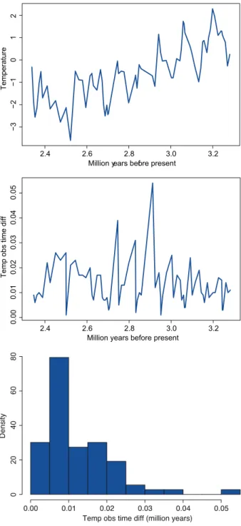
The reason we start analyzing the Pliocene dataset is because it has very interesting interpolation properties, which need some comment and explanation first. There are three variables available in this dataset, temperature anomalies in the sea surface, temperature anomalies in the air, and CO2. These three variables are measured at the same, but unequally spaced, times. Figure 5 shows three graphs. The first one corresponds to the time series of temperatures anomalies in the air. The middle panel includes the observed time differences

(ti − ti−1) versus the final observed time ti and the

last panel corresponds to a histogram of the time differences. Most of the observations were made at a frequency of less than 0.02 million years, with the largest gap of slightly more than 0.05 million years. The median frequency (time difference) is 0.01 mil-lion (10 000) years.

We implemented the interpolation methodology described in Section 4. According to Nieto-Barajas and Sinha (2015) the log-logistic survival function to define the covariance matrix has better performance than the Weibull due to its flexibility to capture slow-er and fastslow-er decays, so the log-logistic will be our choice for all cases considered here. Prior specifica-tions of the Bayesian model are those considered in Nieto-Barajas and Sinha (2015), which are: μ0 = 0, σµ2 = 100, aσ = 2, bσ = 1, aλ = bλ = 1, Aα = 2 and pβ =

0.5. The value of Aα is particularly important since it

constrains the support of parameter α. Larger values of Aα would make the posterior exploration unstable.

(9)

The interpolation process, as described in Section 4, is done via the posterior predictive distribution based on the closest m neighbours. The choice of this parameter plays an important role in the smoothness of the interpolation series. The larger the value of m the smoother the interpolated series becomes.

The best value of m depends on the specific data at hand and its impact is highly dependent on the es-timated correlation function. For the pliocene data, the correlation functions for the three variables (air temperature, SST, and CO2) are included in Figure 6. From the graphs we can see that the correlation

2.4 2.6 2.8 3.0 3.2

−3

−2

−1

01

2

Temperatur

e

2.4 2.6 2.8 3.0 3.2

0.00

0.01

0.02

0.03

0.04

0.05

Temp obs time dif

f

0.00 0.01 0.02 0.03 0.04 0.05

02

04

06

08

0

Temp obs time diff (million years)

Densit

y

Fig. 5. Late Pliocene climate records. Temperature anom-alies in the air. From top to bottom: data, observed time differences versus time, and histogram.

0.0 0.2 0.4 0.6 0.8 1.0

0.

00

.2

0.

40

.6

0.

81

.0

t

S(t

)

0.0 0.2 0.4 0.6 0.8 1.0

0.

00

.2

0.

40

.6

0.

81

.0

t

S(t

)

0.0 0.2 0.4 0.6 0.8 1.0

0.

00

.2

0.

40

.6

0.

81

.0

t

S(t

)

(10)

function for the air temperature variable (left panel) decays fairly fast reaching the value of zero at around one million years. The correlation for SST (middle panel) also presents a very fast decay in the first 0.1 million years but remains almost constant with a very slow rate of decay afterwards. On the other hand, the estimated correlation for CO2 (right panel) has almost no decay, remaining very close to one even after one million years.

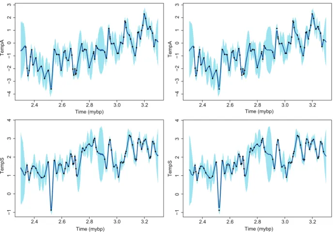
When the correlation function has a fast decay, as is the case of the two temperature variables, the choice of m for interpolation has almost no impact. Figure 7 shows the interpolated series for the two temperature variables with m = 10 closest neighbors and an equal spacing of one and five thousand years, respectively. In all cases the dots correspond to the observed data and the lines to the interpolated data. The shadows correspond to a 95% pointwise

credi-ble interval (CI). As can be seen from the graphs the shadows become larger between two observed data points due to the higher uncertainty in the prediction. The interpolated series at every one thousand years (left column) follows closely the path of the observed points whereas the interpolated series at every five thousand years (right column) has a smoother path, sometimes not reaching the observed points.

As was mentioned before, the estimated correlation function for the CO2 variable is very high. In this case the choice of m has a large impact in the interpolated series. Figure 8 presents the interpolated series using m = 2 (top row) and m = 10 (bottom row) closest neighbors at every one (left column) and five (right column) thousand years, respectively. From this graph the impact of m is clear. For the case of m = 10 at every five thousand years (bottom left panel), the interpolated series follows the path of the observed data but for the

2.4 2.6 2.8 3.0 3.2

−4

−3

−2

−1

3

2

1

0

Temp

A

Time (mybp) 2.4 2.6 2.8 3.0 3.2

−4

−3

−2

−1

3

2

1

0

Temp

A

Time (mybp)

2.4 2.6 2.8 3.0 3.2

−1

0

123

4

Temp

S

Time (mybp) 2.4 2.6 2.8 3.0 3.2

−1

01

23

4

Temp

S

Time (mybp)

(11)

2.4 2.6 2.8 3.0 3.2

200

30

04

00

500

CO

2

Time (mybp)

2.4 2.6 2.8 3.0 3.2

200

300

400

500

CO

2

Time (mybp)

2.4 2.6 2.8 3.0 3.2

200

300

400

500

CO

2

Time (mybp) 2.4 2.6 2.8 3.0 3.2

200

300

400

500

CO

2

Time (mybp)

Fig. 8. Late Pliocene climate records. Interpolated CO2 data at every one (first column) and five (second column) thousand years using m = 2 (top row) and m = 10 (bottom row) closest neighbors. Full dots correspond to observed data, lines to interpolated series, and shadows to 95% CI.

non observed times the interpolated series quickly goes down/up to an average value. However this over smoothing effect is not present when m = 2 for the same spacing of five thousand years (top left panel). Given the large correlation in this CO2 variable, it is preferable to interpolate using the smaller value of m = 2 neighbors to avoid over smoothing.

We move on to the Paleozoic data. There are two variables available, temperature anomalies and CO2. These two variables have not been measured at the same times and are not equally spaced. Moreover, the temperature was recorded from 265 to 303.5 million years before the present, whereas CO2 was measured from 273.3 to 300.2 million years before the present. The observation time for the CO2 vari-able has a shorter span and its range lies within that of the temperature. See also the two panels in the first column of Figure 9. The frequency with which these two variables were measured is also shown in

Figure 9 (middle and right columns) where we plot the observed time differences. For the CO2 variable (bottom row), most of its observations were measured at a frequency less than 0.5 million years, whereas temperature (top row) was measured at more dis-persed frequencies with most of the observations made at time differences larger that 0.5 million years.

(12)

Fig. 9. Late Paleozoic deglaciation data. From left to right: data, observed time dif

ferences versus time, and histogram. From top to bottom: temperature anomalies, CO

265

270

275

280

285

290

295

300

500 1500

2500 3500

CO 2

26

52

70

27

52

80

28

52

90

29

53

00

0.5 1.0

1.5

CO 2

obs time diff

0.

51

.0

CO

2

obs time diff (million years)

Density

0 1 2 3 4

265

270

275

280

28

52

90

29

53

00

−6 −4 −2 0 2 4 6

Temperature

265

270

275

280

285

29

02

95

30

0

0.5 1.0 1.5 2.0 2.5 3.0

Temp obs time diff

0.5

1.0

1.

52

.0

2.

53

0.0 0.5 1.0 1.5 2.0 2.5 3.0

Temp obs time diff (million years)

(13)

270 280 290 300

−1

0−

51

0

5

0

Temp

A

Time (mybp) 270 280 290 300

−1

0−

51

0

5

0

Temp

A

Time (mybp)

270 280 290 300

0

1000

2000

3000

4000

CO

2

Time (mybp)

270 280 290 300

01

000

2000

3000

4000

CO

2

Time (mybp)

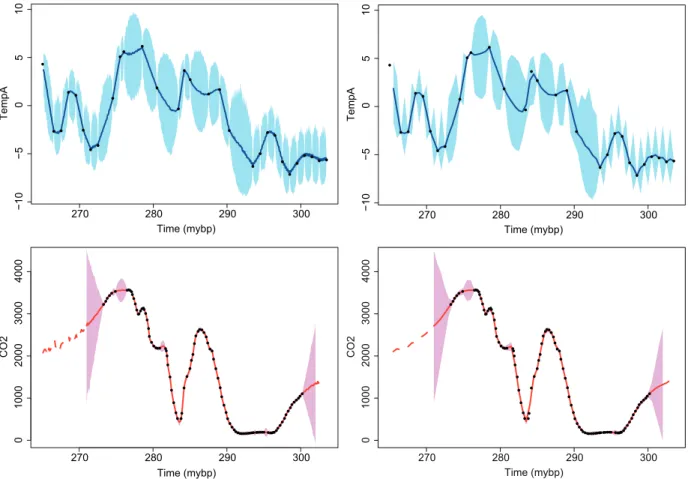
Fig. 10. Late Pliocene climate records. Interpolated data using m = 10 closest neighbors at every 0.1 (first column) and 0.5 (second column) million years. Temperature (top row) and CO2 (bottom row). Full dots correspond to observed data, lines to interpolated series, and shadows to 95% CI.

million years, the predicted series shows a huge uncertainty that increases as we move away. Strictly speaking, for these times beyond the observed time range we are doing an extrapolation of the time se-ries, and going far beyond the limits produces a huge uncertainty. The shadows in the two bottom panels for the times beyond the observed range increase in size very fast as we go away. Note that in the graph the shadows were only included for the closest ex-trapolated times to avoid increasing the scale of the graph. For the further away time points we decided to report only the point predicted values and are shown as dashed lines in the graphs.

Finally, we analyze the marine isotope stage dataset. There are three variables available: tem-perature anomalies, carbon dioxide, and methane. Figure 11 includes the observed time series for these three variables (first column). The middle and right

panels report the observed time differences vs. time and a histogram, respectively for the three variables. Broadly speaking, temperature and CH4variables were measured at an increasing frequency, that is, they were measured very frequently close to present and less frequent as we go back in time up to 800 thousand years. The CO2 variable, on the other hand, has a reversed path in terms of frequency it was not measured very often close to present time, but was measured more frequently as we go back in time. The maximum gap between measurements is 1.36 thousand years for temperature, 6.02 for the CO2 variable, and 3.46 for the CH4 variable. The median observed time differences are 0.06, 0.58 and 0.31 thousand years, respectively for the three variables.

(14)

0 200 400 600 800 −10 −5 0 5

Temperature 0 200 40 06 00 80 0 0.0 0.2 0.4 0.6 0.8 1.0 1.2 1.4

Temp obs time diff

0.0 0. 20 .4 0. 60 .8 1. 01

Temp obs time diff (thousand years)

Density 0 1 2 3 4 5 6 0 200 400 60 08 00 180 200 220 240 260 280 300 C02

Thousand years before presen

t 0 200 400 60 08 00

6 5 4 3 2 1 0

C02 obs time diff

t 5 4 3 2 1 0 0.0 0.2 0.4 0.6 0.8 Density

C02 obs time diff (thousand years)

0 200 40 06 00 80 0 400 500 600 700 800 900 CH4

t 02 00 40 06 00 80 0 0.0 0.5 1.0 1.5 2.0 2.5 3.0 3.5

CH4 obs time diff

0.0 0.5 1. 01 .5 2. 02 .5 3. 0.0 0.5 1.0 1.5

CH4 obs time diff (thousand years)

Density

Fig. 1

1. EPICA

dome C ice core 800 thousand years data. From left to right: data, observed time dif

ferences versus time, and histogram. From top to bottom: temperature

anomalies, CO

2

, CH

4

(15)

Fig. 12. EPICA dome C ice core 800 thousand-years data. Interpolated data using m = 10 closest neighbors at every 100 (first column) and 500 (second column) years. Temperature (top row), CO2 (middle row) and CH4 (bottom row). Lines correspond to interpolated series and shadows to 95% CI.

0 200 400 600 800

−1

0−

50

5

Time (tybp)

0 200 400 600 800

−1

0−

50

5

Time (tybp)

Temp

0 200 400 600 800

160

180

200

220

240

260

280

300

CO

2

Time (tybp)

0 200 400 600 800

160

180

200

22

02

40

260

280

300

Time (tybp)

CO

2

0 200 400 600 800

30

04

00

500

600

700

800

Time (tybp)

CH4

0 200 400 600 800

30

04

00

500

600

700

800

Time (tybp)

CH4

0.1 and 0.5 thousand years. The interpolated series together with a 95% credible interval are presented in Figure 12. Note that the credible intervals are larger in regions were the observed data are more spaced (less frequently measured), that is, closer to 800 thousand years for the temperature (top row) and

methane (bottom row) variables, and closer to zero for the carbon dioxide (middle row) variable.

(16)

with a 95% CI are presented in Figure 12. Note that CIs are larger in regions where the observed data are more spaced (less frequently measured), that is, closer to 800 000 years for the temperature (top row) and methane (bottom row) variables, and closer to zero for the CO2 (middle row) variable.

6. Concluding remarks

In this article we collected four important data sets for climate change study. Three of these datasets are representative of the paleoclimate covering periods from marine isotope stage, passing by the late Plio-cene up to the late Paleozoic deglaciation.

We used a Bayesian statistical method to inter-polate the datasets and produced equally spaced observations in the observed range. The original data as well as the interpolated values are available as supplementary material.

Interpolated values include point predictions (predictive means) and quantiles of order 2.5% and 97.5%. The latter two can be used as the lower and upper limits, respectively, to produce 95% CIs as those shown in Figures 7, 8, 10 and 12.

One important challenge that is worth exploring in paleoclimate statistical research is to consider the age-uncertainty into the model, that is, to produce a joint modeling of the climatic variable as well as the observation time. This would produce a better model since all sources of uncertainty would be taken into account.

Acknowledgments

This research was supported by CONACyT grant 244459 and the Asociación Mexicana de Cultura, A.C.

References

Bayraktar H. and Turalioglu F.S., 2005. A Kriging-based approach for locating a sampling site in the assessment of air quality. Stoch. Environ. Res. Risk A. 19, 301-305. DOI: 10.1007/s00477-005-0234-8.

Bernardo J.M. and Smith A.F.M., 2000. Bayesian theory. Wiley, New York, 610 pp.

British Antarctic Survey, 2014. Ice cores and climate change. National Environment Research Council. Available at: https://www.bas.ac.uk/data/our-data/ publication/ice-cores-and-climate-change/

Chang J.T., 2012. Stochastic processes. Technical report.

Department of Statistics, Yale University. Available at: http://www.stat.yale.edu/~pollard/Courses/251. spring09/Handouts/Chang-notes.pdf

DeGroot M.H., 2004. Optimal statistical decisions. Wiley, New Jersey, 489 pp.

Eckner A., 2012. A framework for the analysis of unevenly spaced time series data. Preprint. Available at: http:// www.eckner.com/papers/unevenly_spaced_time_se-ries_analysis.pdf

Handcock M.S. and Stein M.L., 1993. A Bayesian analysis of kriging. Technometrics 35, 403-410.

DOI: 10.2307/1270273

Hansen J., Ruedy R., Sato M. and Lo K., 2010. Global sur-face temperature change. Rev. Geophys. 48, RG4004. DOI: 10.1029/2010RG000345

Jouzel J., Masson-Delmotte V., Cattani O., Dreyfus G., Falourd S., Hoffmann G., Minster B., Nouet J., Barnola J.M., Chappellaz J., Fischer H., Gallet J.C., Johnsen S., Leuenberger M., Loulergue L., Luethi D., Oerter H., Parrenin F., Raisbeck G., Raynaud D., Schilt A., Schwander J., Selmo E., Souchez R., Spahni R., Stauffer B., Steffensen J.P., . Stenni B, Stocker T.F., Tison J.L., Werner M. and Wolff E.W., 2007. Orbital and millennial antartic climate variability over the past 800 000 years. Science 317, 793-796.

DOI: 10.1126/science.1141038

Keeling R.F., Piper S.C., Bollenbacher A.F. and Walker S.J., 2008. Atmospheric CO2-curve samples collected at the South Pole. Carbon Dioxide Research Group, Scripps Institution of Oceanography (SIO), University of California. Available at: http://cdiac.ornl.gov/ftp/ trends/co2/sposio.co2

Loulergue L., Parrenin F., Blunier T., Barnola J.-M., Spahni R., Schilt A., Raisbeck G. and Chappellaz J., 2007. New constraints on the gas age - ice age differ-ence along the EPICA ice cores, 0-50 kyr. Clim. Past 3, 527-540.

DOI: 10.5194/cp-3-527-2007

Loulergue L., Schilt A., Spahni R., Masson-Delmotte V., Blunier T., Lemieux B., Barnola J.M., Raynaud D., Stocker T.F. and Chappellaz J., 2008. Orbital and millennial-scale features of atmospheric CH4 over the past 800 000 years. Nature 453, 383-386.

DOI: 10.1038/nature06950

(17)

years before present. Nature 453, 379-381. DOI: 10.1038/nature06949

MacFarling Meure C., Etheridge D., Trudinger C., Steele P., Langenfelds R., van Ommen T., Smith A. and El-kins J., 2006. Law Dome CO2, CH4 and N2O ice core records extended to 2000 years BP. Geophys. Res. Lett. 33, L14810. DOI: 10.1029/2006GL026152

Montanez-Boti M.A., Foster G.L., Chalk T.B., Rohling E.J., Sexton P.F., Lunt D.J., Pancost R.D., Badger M.P.S. and Schmidt D.N., 2015. Plio-Pleistocene cli-mate sensitivity evaluated using high-resolution CO2 records. Nature 518, 49-54. DOI: 10.1038/nature14145 Montanez I.P., Tabor N.J., Niemeier D., DiMichele W.A.,

Frank T.D., Fielding C.R., Isbell J.L., Birgenheier L.P. and Rygel M.C., 2007. CO2-forced climate and veg-etation instability during late Paleozoic deglaciation. Science 315, 87-91. DOI: 10.1126/science.1134207 Mudelsee M. Climate time series analysis: Classical

sta-tistical and bootstrap methods. Springer, New York, 454 pp.

Nieto-Barajas L.E. and Sinha, T., 2015. Bayesian interpo-lation of unequally spaced time series. Stoch. Environ. Res. Risk A. 29, 577-587.

DOI: 10.1007/s00477-014-0894-3

Parrenin F., Barnola J.-M., Beer J., Blunier T., Castellano E., Chappellaz J., Dreyfus G., Fischer H., Fujita S., Jouzel J., Kawamura K., Lemieux-Dudon B., Loul-ergue L., Masson-Delmotte V., Narcisi B., Petit J.-R., Raisbeck G., Raynaud D., Ruth U., Schwander J., Severi M., Spahni R., Steffensen J. P., Svensson A., Udisti R., Waelbroeck C. and Wolff E., 2007. The EDC3 chronology for the EPICA Dome C ice core. Clim. Past 3, 485-497. DOI: 10.5194/cp-3-485-2007 Polanco-Martínez J.M. and Faria S.H., 2015. Towards

a new statistical tool for analyzing unevenly spaced paleoclimate time series. Preprint. Available at: https:// www.researchgate.net/publication/280084942_To-wards_a_new_statistical_tool_for_ analyzing_uneven-ly_spaced_paleoclimate_time_series

Rasmussen C.E. and Williams C.K.I., 2006. Gaussian processes for machine learning. MIT Press, Massa-chusetts, 272 pp.

Renard B., Lang M. and Bois P., 2006. Statistical analysis of extreme events in a nonstationary context via a Bayesian framework. Stoch. Environ. Res. Risk A. 21, 97-112. DOI: 10.1007/s00477-006-0047-4

Rehfeld K. and Kurths, J., 2014. Similarity estimators for irregular and age-uncertain time series. Clim. Past 10, 107-122. DOI: 10.5194/cp-10-107-2014

Robinson P.M., (1977. Estimation of a time series model from unequally spaced data. Stoch. Proc. Appl. 6, 9-24. DOI: 10.1016/0304-4149(77)90013- 8

Schulz M. and Mudelsee, M., 2002. REDFIT: Estimating red noise spectra directly from unevenly spaced pa-leoclimatic time series. Comput. Geosci. 28, 421-426. Schulz M. and Stattegger, K. (1997). SPECTRUM: spec-tral analysis of unevenly spaced paleoclimatic time series. Computers and Geosciences 23, 929-945. Smith A. and Roberts G., 1993. Bayesian computations

via the Gibbs sampler and related Markov chain Monte Carlo methods. J. R. Stat. Soc. B 55, 3-23.

DOI: 10.2307/2346063

Van de Wal R.S.W., de Boer B., Lourens L.J., Kohler P. and Bintanja R., 2011. Reconstruction of a continuous high-resolution CO2 record over the past 20 million years. Clim. Past 7, 1459-1469.