Semiautomated segmentation of bone marrow biopsies images based on texture features and Generalized Regression Neural Networks

Semiautomated segmentation of bone marrow biopsies images based on

texture features and Generalized Regression Neural Networks

Meschino Gustavo (1,2), Passoni Lucía Isabel (1), Moler Emilce (2)

(1)

Laboratorio de Bioingeniería – (2) Laboratorio de Procesos y Medición de Señales Facultad de Ingeniería, Universidad Nacional de Mar del Plata

Juan B. Justo 4302 - B7608FDQ Mar del Plata gmeschin@fi.mdp.edu.ar

Abstract

This work presents preliminary results of a method for semi-automatic detection of fat and hematopoietic cells as well as trabecular surfaces in bone marrow biopsies, in order to calculate the percentage of each type of tissue or cell area in relation to the whole area.

Experimental results using selected clinical cases are presented. Twenty six biopsies were used, presenting varied distributions of cellularity and trabeculae topography. The approach is based on Digital Image Processing techniques and a Neural Network used for classification using textural features obtained from biopsies images. Results were improved with Mathematical Morphology filters.

The algorithm produces highly satisfactory results. The method was shown to be faster and more reproducible than conventional ones, like region growing, edge detection, split and merging.

The results from this computer-assisted technique are compared to others obtained by visual inspection by two expert pathologists, and differences of less than 9 % are observed.

Keywords

1. Introduction

One of the most interesting fields in Digital Image Processing is the segmentation of an image into its different objects (Gonzalez and Woods, 1993). Segmentation plays a vital role in numerous biomedical imaging applications, such as the quantification of tissue volumes, diagnosis, localization of pathologies, study of anatomical structures and others (Glasbey 1995). The segmentation techniques can be divided into two groups: techniques based on contour detection which search for local grey level discontinuity in the image and those involving region growing which seek homogeneous image parts according to statistical measurements such as grey level and texture. The segmentation process of medical images is a difficult task to be accomplished in digital image processing (Chalama 1997).

Histopathology is an area normally considered in purely descriptive terms. However, a quantitative approach may bring it to more solid grounds. This is definitely true for bone pathologies (Frisch 1985). Changes in the amount of total bone and osteoid, together with the activity of fat and hematopoietic cells as well as trabecular surfaces, are probably the most important features in metabolic bone disease (Bullough 1990). The manual analysis of bone marrow is tedious and a time-consuming task that can be simplified by means of an automatic method (Revell 1983). With this automation better statistical information can be obtained (Clermonts 1985).

The goal of this work is the building of a tool to support pathology reports generation where the quantification and classification biopsies items are present. The use of a computational method to achieve classification and cell counting is very useful to help in qualitative and quantitative aspects of final diagnosis.

Numerous segmentation methods for cell images have been proposed, most of them trying to detect and separate different types of cells (Wu 1999, Sobrevilla 1999, De Medeiros 2001, Park 1997). Although they are useful antecedents of this work, the advantage of the method we propose is that it also produces good results for segmentation of trabecular surfaces.

The method consists in the application of a semi-automatic simple pattern classification algorithm based on the texture that images present.

Texture segmentation is a long established research field in image processing (Russ 1995). Texture means the subjective impression of the appearance of a surface. The classification based on texture feature values has become the essential technique for the treatment of some medical images (Baeg 1998, Serón 2002, Kneitz 1996, Nasser Esgiar 1998). Main research fields search for well-suited texture feature calculation methods and appropriate classification techniques.

For texture recognition, the image is divided into small sub-images. From the gray levels of each sub-image, textural features are computed. Many methods for the computation of these have been proposed so far (Singh 2001, Singh 2002). These methods can be divided into some main groups, such as statistical features, frequency-domain based features, fractal features and those derived from Wavelets and Gabor decomposition.

1994, Cross 1993, Dougherty 2001) was tried in an earlier stage, but the preliminary segmentation obtained was not successful in the marrow biopsies images.

Classical automatic schemes for classification like K-means and Fuzzy-C-means did not give satisfactory results when applied to marrow biopsies images. Consequently we propose a semi – automatic mapping process achieved with Generalized Regression Neural Networks (GRNN).

This work compares the results obtained using statistical (Gray level co-occurrence matrix) and frequency-domain (spectral power density) based features.

In a second stage of the method, morphological filters, derived from Mathematical Morphology theory, were used to improve the segmentation. Mathematical Morphology refers to a branch of nonlinear image processing and analysis, which focuses on the geometric structures within an image (Serra 1982). It emerged as a general theory to providing a unified approach in order to deal with problems in Medicine, Biology, and many other fields and can be applied in a satisfactory way to the resolution of fat cells segmentation problems (Dougherty 1992).

The proposed method is described in the next sections.

2. Materials and Methods

2.1. Image Acquisition

The images were obtained from bone marrow biopsies. They were chosen among normal samples and bone marrow biopsies that showed different disorders.

This work is based on twenty-six images. These were obtained from an Optic Microscope Medilux-12 with a TC Plan Achromat 4X objective, N.A. 0.10 and digitized with a CCD Hitachi KP-C550 color camera. This camera has an effective pixel dimension of 682 (H) x 492 (V) and a wavelength range of 400 to 700 nm. It supports a video resolution of 430 TV scan lines which was sufficient to capture biopsy images of 640 x 480 pixels from the live video by a PC. After selecting the area of interest, a single image is recorded in each case.

The images were saved on Windows Bitmap format and converted to 8-bit gray scale.

2.2. Generalized Regression Neural Networks

The mapping process is achieved using the Generalized Regression Neural Networks (GRNN) proposed by Specht (Specht 1991). The GRNN architecture is rather similar to the Probabilistic Neural Networks, also known as Radial Basis Network Functions (RBF).

The GRNN trains faster than other multilayer architectures and they model arbitrary non – linear functions efficiently. However they demand larger computational availabilities and a longer recall lapse than the wide known multilayer perceptron.

information to the intermediate layer, the cells of the hidden layer are activated with a function of the distance between the input pattern and the synaptic weights, stored in each cell (called centroid) via a radial gaussian function.

Each neuron j of the hidden layer stores a vectorial cji, the centroid, whose distances rj it is

calculated as the euclídean distance that separates to the vector of entrance xi of the centroid:

2 2

2

)

(

j

j

x

c

x

c

r

=

−

=

∑

−

where xi = net inputs and yi = hidden layer outputs

The output of the neuron yj is calculated applying a radial function, term that is applied to

symmetrical functions, usually the gaussian:

2 2 2 /

)

(

φ

e

r

=

The output of the hidden neuron j is shown in Equation 3.

∑

=

j ji i c x j

e

y

( σ

Ec. 3

Each node of the hidden layer specializes on an input region space and the whole set of input cells must totally cover the interest region.

The outputs of the hidden neurons, each corresponding to a space region pattern are weighted and normalized previously to be fed to the output layer. The transfer functions of the output layer neurons are lineal, and they calculate the pondered and normalized sum of the hidden layer output (Equation 4).

∑

∑

2.2. Segmentation Process

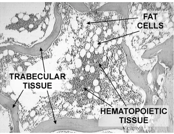
The different types of tissues regions to identify are shown on Figure 1.

Figure 1: Typical image of a bone marrow biopsy.

The expert chooses N pixels, at least three, which correspond to each texture class to detect. The goal is to detect three classes corresponding to trabeculae surface, hematopoietic and fat cells.

Once the sample pixels are chosen, texture features corresponding to the region that surrounds each pixel are calculated. The size of the analysis region should be chosen appropriately, as it will be explained later on. The method was developed experimenting with two types of features:

• Statistical Features: they are based on different operations on Gray Level Co-occurrence Matrix (GLCM). After evaluating several feature combinations the vector was constructed as: H = [cnth cntv cntd engh engv engd eph epv epd maxh maxv maxd mean], where:

- cnth, cntv, cntd: Contrast at GLCM in horizontal (0º), vertical (90º) and diagonal (45º) direction respectively.

- engh, engv, engd: Energy (order 0 differential moment) at GLCM in the same directions. - eph, epv, epd: Entropy at GLCM in the same directions.

- maxh, maxv, maxd: Maximal Probability at GLCM in the same directions. - mean: Ratio of gray mean value to maximum of the range.

• Frequency Features: the vector in this case is composed by the values obtained after application of Fourier Transform and the later Spectral Density Power calculation. The values of the first and fourth quadrants of the transform are arranged in a vector.

Subsequently, the image is processed by regions of the same size. The successive regions could be overlapped. The same type of texture features used at the sample pixels are calculated for each region.

Let x be the feature vector of the region that is being analyzed. This vector will be the input of the trained GRNN. The output given by the network will be a number in the range [1, 256] which indicates the gray level for the classification image.

Thus the classification image is created. This image will be processed to have only three gray values, making a simple transformation: the values in [1, 64] will be transformed to 1, the values in [65, 192] will be transformed to 127 and the values in [193, 256] will be transformed to 256. The final image is obtained, with 3 gray intensities.

Parameters are chosen empirically using the set of images:

• Amount of sample pixels: The number of prototypes patterns characterizing every class to segment.

• Region size: The size of the window where texture features are calculated.

• Region Overlapping: It defines the window displacement.

• Features Vector: It can be calculated by Fourier Transform of the region or by statistical analysis (co-occurrence matrix).

• The spread value: an internal parameter of the GRNN.

2.3. Post-processing

The segmented image may contain wrongly identified regions. This error is mainly due to the fact that in some regions more than one texture may be present. To improve the accuracy of the segmentation it is useful to apply some Mathematical Morphology filters.

The application of the different Morphological filters should be interactively indicated by the user, always matching the segmentation image with the original image.

The options are:

• Dilation of one of the classes: it allows enlarging some of the segmented regions without losing their shape.

• Erosion of one of the classes: it achieves the opposite effect to the dilation, diminishing the area covered by the class that is indicated.

• Closing: if during the detection erroneous holes appear within one of the classes, this operation will close them.

• Elimination of small areas: it is made by combination of morphological filters to eliminate objects of a certain connectivity whose area is smaller than a given threshold.

2.4. Area Calculation

interest (ROI) of the image where there are not artifacts, and the segmentation has been satisfactory. The ROI have a polygonal shape.

Given the region of interest, the class area percentages are calculated (trabecular tissue, fat cells, hematopoietic tissue), according to the next expression:

Amount of class i pixels % Class i Area 100

Amount of ROI pixels

= ×

2.5. Implementation

The proposed technique was implemented on MatLab© 6.5. The Morphological Filters was extracted from the SDC Morphology Toolbox©.

To facilitate the test stage and to have an appropriate way to interact with pathologists, a user– friendly interface was constructed. This shows the original image, the segmentation image and the results of the application of every filter.

The pathologist observes morphological filters with appropriate medical sentences that are easily understood by the operator such as “Close of holes the trabeculae region”, “Increase fat area” and “Decrease cellularity area”.

3. Results

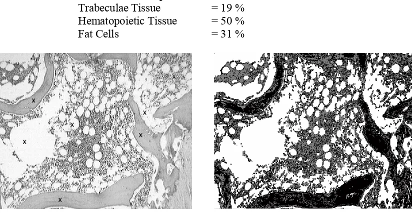
Figure 2 shows the step sequence of the proposed method for one sample image. Figure 2 (a) shows the original image, with the pixels of three classes selected by a user. Figure 2 (b) shows the segmented image using frequency texture features. Figure 2 (c) presents the improvement achieved by morphological methods. Figure 2 (d) shows the chosen region for the calculation of areas. The numerical results obtained for this example are:

Trabeculae Tissue = 19 % Hematopoietic Tissue = 50 % Fat Cells = 31 %

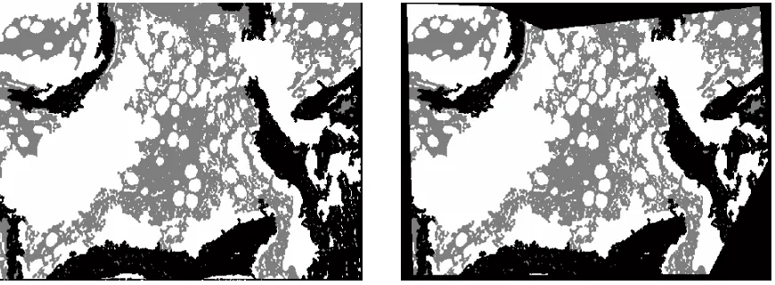
(c) Improvement achieved by morphological methods.

(d) Chosen region for calculation of areas.

Figure 2: Steps sequence of the proposed method.

The same process was applied to a whole set of images. Table I shows the obtained values by the proposed method and the results that the pathologists have reported. For comparison, the average of the quantities they gave is taken, since these quantities varied as much as 35 %, which shows the subjectivity of the visual analysis.

To make a comparison between the results of the pathologists, the ones obtained using statistical features and the ones obtained using frequency features, three vectors were constructed for each image, where its components are the percentages obtained for each class (trabeculae, fat and hematopoietic cells).

In order to evaluate the difference between the pathologists results vector and the results obtained with the presented method, Euclidean vectorial distances were calculated. To make this value a significant index, it was necessary to normalize it. The normalization was calculated as:

P SF

Min Max

(V , V )

% %

(V ,V )

d SE

d

=

P FF

Min Max

(V , V )

% %

(V ,V )

d FE

d

=

where:

P

V = Vector of results suggested by the pathologist.

SF

V = Vector of results obtained using statistical features.

FF

V = Vector of results obtained using frequency features.

Min

V = Vector of minimal values of the range (0, 0, 0).

Max

The errors are shown in the last two columns in Table I. Empty cells indicate that the method didn’t work suitably.

Pathologist Statistical Features

Frequency

Features SE % FE %

Trabeculae 11 16 17

Fat 87 80 80

Image 1

Hematopoietic 2 4 3

5% 5%

Trabeculae 18 26 24

Fat 79 73 73

Image 2

Hematopoietic 3 1 3

6% 5%

Trabeculae 18 24

Fat 77 71

Image 3

Hematopoietic 5 5

5%

Trabeculae 33 32

Fat 60 63

Image 4

Hematopoietic 7 5

2%

Trabeculae 70 54 75

Fat 5 4 5

Image 5

Hematopoietic 25 42 20

13% 4%

Trabeculae 64 49 66

Hematopoietic 6 3 2

Image 6

Fat 30 48 32

14% 3%

Trabeculae 60 57

Hematopoietic 8 10 Image 7

Fat 32 33

2%

Trabeculae 35 36 38

Hematopoietic 35 39 39

Image 8

Fat 30 25 23

4% 5%

Trabeculae 26 22 27

Hematopoietic 54 57 51

Image 9

Fat 20 21 22

3% 2%

Trabeculae 24 17 23

Hematopoietic 52 62 52

Image 10

Fat 24 21 25

7% 1%

Trabeculae 26 15

Hematopoietic 53 33

Image 11

Fat 21 52

22%

Trabeculae 19 15 22

Hematopoietic 47 46 47

Image 12

Fat 34 39 31

4% 2%

Trabeculae 20 32 17

Hematopoietic 57 48 51

Image 13

Fat 23 20 32

9% 6%

Trabeculae 21 24 20

Hematopoietic 39 49 50

Image 14

Fat 40 27 30

10% 9%

Trabeculae 17 18 15

Hematopoietic 41 50 46

Image 15

Fat 42 32 39

8% 4%

Trabeculae 19 19 12

Hematopoietic 27 47 39

Image 16

Fat 54 34 49

16% 9%

Trabeculae 15 20

Hematopoietic 45 49

Image 17

Fat 40 31

6%

Trabeculae 19 16 16

Hematopoietic 35 44 38

Image 18

Fat 46 40 46

6% 2%

Trabeculae 12 21 30

Hematopoietic 20 31 27

Image 19

Fat 68 48 43

14% 18%

Trabeculae 10 18 15

Hematopoietic 18 29 21

Image 20

Fat 72 53 64

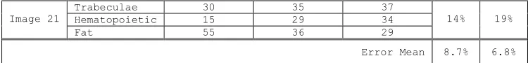
Trabeculae 30 35 37

Hematopoietic 15 29 34

Image 21

Fat 55 36 29

14% 19%

Error Mean 8.7% 6.8%

Table I: Numerical results

4. Discussion

The automatic bone marrow microscope analysis presents several difficulties due to the diversity of elements appearing in this kind of images (Baak 1991). The different types of tissues and cells frequently are overlapped and the presence of artifacts complicates the problem. In most situations, this difficulty forces the use of very specific segmentation algorithms for each task. This makes bone marrow image segmentation a difficult and challenging problem(Liu 1999).

The accuracy of segmentation mainly depends on the selection of good parameters. After experiencing with images, some criteria can be determined for the choice of parameters.

• Amount of sample pixels: It is chosen keeping in mind that a big quantity of sample pixels possibly improves the classification, but it will increase the processing time.

• Size of the region: if it is small, processing time will decrease, but it is risky in the sense that different textures can not be segmented correctly. On the other hand, if it is too big, apart from increasing the calculation time considerably, the probability of the analysis region containing more than one texture increases, surely leading to classification errors.

• Region Overlapping: if the window of analysis is moved in a single pixel step manner, a lengthy processing time will be required, and the result will not be notably better than the result obtained using bigger displacements. For example, moving the window by two pixels decreases calculations by one half, and the classified regions will have a size of 2 x 2 pixels, what allows an equally successful segmentation.

• Calculated Features: features calculated in the frequency domain leads to a noisier segmentation, but after a simple post-processing, acceptable results are achieved. The unquestionable advantage of the frequency domain is the fact that processing time decreases drastically if compared with co-occurrence features. The statistical features based on gray level co-occurrence matrix results in a clearer classification, but processing time increases considerably.

As mentioned before, the results obtained were compared to the reports obtained by visual inspection performed by two pathologists. The discrepancy between the two pathologists’ reports justifies the use of the method we propose which gives differences smaller than 9 % if compared with the average of the results given by experts.

A tool providing such capabilities can reduce counting error produced by a subjective analysis and can shorten the time taken by manual counting. Besides that, it avoids inter and intra observer variability.

A need for automation is evident. But once optimized the sequence to follow for the processing of an image, a quick segmentation and area calculation process is obtained. It would facilitate the professional's work, decreasing diagnosis errors and minimizing subjectivity in bone marrow analysis.

For future work, it will be of interest to make new comparisons applying the presented method to images obtained at different magnifications and stained with different techniques.

5. Acknowledgements

The authors thank Dr. Ulises Zanetto and Dr. Fernando Pagani, expert pathologists, for providing instrumental and the histologic material apart from their helpful and enlightening discussion.

6. References

Baak J (1991): Manual of Quantitative Pathology in Cancer Diagnosis and Prognosis. New York, Springer-Verlag.

Baeg S, Popov A, Kamat V, Batman S, Sivakumar K, Kehtarnavaz N, Dougherty ER, Shah RB (1998): Segmentation of Mammograms into Distinct Morphological Texture Regions. IEEE Symposium on Computer-Based Medical Systems, Lubbock, June 1998.

Bullough PG, Bansal M, DiCarlo EF (1990): The tissue diagnosis of metabolic bone disease. Role of histomorphometry. Orthop Clin North Am; 21:65-79.

Chalama V, Kim Y (1997): A methodology for evaluation of boundary detection algorithms on medical images. IEEE Trans Med Imag; 16:642-652.

Clermonts E, Birkrnhager–Frenkel D (1985): Software for bone histomorphometry by means of a digitizer. Comput Methods Programs Biomed; 21:185-94.

Cross S (1994): The Application of Fractal Geometric Analysis to Microscopic Images. Micron; 25 (1):101-113

Cross S, Rogers S, Silcocks PB, Cotton DWK (1993): Trabecular bone does not have a fractal structure on light microscope examination. J Pathol; 170:311-313.

De Medeiros Martins A, Duarte Dória Neto A, Medeiros Brito A, Sales A, Jane S (2001): Texture based segmentation of cell images using neural networks and mathematical morphology. Proceedings of IJCNN’2001, Washington, D.C., IEEE / Omnipress, pp. 2489-2494.

Dougherty E (1992): An Introduction to Morphological Image Processing. Washington, SPIE. Dougherty G, Henebry, G (2001): Fractal signature and lacunarity in the measurement of the texture

of trabecular bone in clinical CT images. Med Eng Phys; 23:369-380.

Glasbey C, Horgan, G (1995): Image Analysis for the Biological Sciences. New York, John Wiley & Sons.

Gonzalez R, Woods R (1992): Digital Image Processing. USA, Addison – Wesley, pp. 458-465. Haralick RM, Shanmugan K, Dinstein I (1973): Textural features for image classification. IEEE

Transactions on Systems, man and Cybernetics; SMC-3:610-621.

Haykin S (1999): Neural Networks: A Comprehensive Foundation. Prentice-Hall.

Kneitz S, Ott G, Albert R, Schindewolf T, Muller-Hermelink HK, Harms H (1996): Differentiation of Low Grade Non-Hodgkin's Lymphoma by Digital Image Processing. Analyt Quant Cytol Histol; 18:121-128.

Liu Z, Liew HL, Clement JG, Thomas DL (1999): Bone Image Segmentation. IEEE Trans Biomed Eng; 46 (5):565-573.

Nasser Esgiar A, Raouf N, Naguib G, Bennett MK, Murray A (1998): Automated Feature Extraction and Identification of Colon Carcinoma. Analyt Quant Cytol Histol; 20:297-301

Park JS, Keller JM (1997): Fuzzy Patch Label Relaxation in Bone Marrow Cell Segmentation. Proc. IEEE International Conference on Systems, Man, and Cybernetics, Orlando, FL., October 1997, pp. 1133-1138.

Revell P (1983): Histomorphometry of bone. J Clin Pathol Review; 36: 1323-1331. Russ, JC (1995): The Image Processing Handbook. USA, CRC Press, pp. 361-367

Serón D, Moreso F, Gratin C, Vitriá J, Condom E, Grinyó JM, Alsina J (2002): Automated Classification of Renal Interstitium and Tubules by Local Texture Analysis and a Neural Network. Analyt Quant Cytol Histol; 24:147-153.

Serra J (1982): Image Analysis and Mathematical Morphology. London, Academic Press.

Singh M, Singh S (2001): Evaluation of Texture Methods for Image Analysis. Proc. 7th Australian and New Zealand Intelligent Information Systems Conference, Perth, November 2001.

Singh M, Singh S (2002): Spatial Texture Analysis: A Comparative Study. Proc. 15th International Conference on Pattern Recognition (ICPR'02), Quebec, August 2002.

Sobrevilla P, Keller J, Montseny E (1999): White Blood Cell detection in Bone Marrow images. Proc. of 18th NAFIPS International Conference, New York, USA, June 1999, pp 403-407. Specht, D (1991): A General Regression Neural Network. IEEE Transactions on Neural Networks,

2 (6): 588-576.

Tou J, Gonzalez R (1974): Pattern Recognition Principles. New York, Addison – Wesley.