www.nonlin-processes-geophys.net/20/683/2013/ doi:10.5194/npg-20-683-2013
© Author(s) 2013. CC Attribution 3.0 License.
Nonlinear Processes
in Geophysics
A top-down model to generate ensembles of runoff from a large
number of hillslopes
P. R. Furey1, V. K. Gupta2, and B. M. Troutman3 1NorthWest Research Associates, Boulder, CO, USA
2Dept. of Civil, Environmental and Architectural Engineering, Cooperative Institute for Research in Environmental Sciences, University of Colorado, Boulder, CO, USA
3Lakewood, CO, USA
Correspondence to: P. R. Furey (prfurey@gmail.com)
Received: 31 October 2012 – Revised: 13 June 2013 – Accepted: 30 July 2013 – Published: 25 September 2013
Abstract. We hypothesize that total hillslope water loss for
a rainfall–runoff event is inversely related to a function of a lognormal random variable, based on basin- and point-scale observations taken from the 21 km2 Goodwin Creek Experimental Watershed (GCEW) in Mississippi, USA. A top-down approach is used to develop a new runoff gener-ation model both to test our physical-statistical hypothesis and to provide a method of generating ensembles of runoff from a large number of hillslopes in a basin. The model is based on the assumption that the probability distributions of a runoff/loss ratio have a space–time rescaling property. We test this assumption using streamflow and rainfall data from GCEW. For over 100 rainfall–runoff events, we find that the spatial probability distributions of a runoff/loss ratio can be rescaled to a new distribution that is common to all events. We interpret random within-event differences in runoff/loss ratios in the model to arise from soil moisture spatial vari-ability. Observations of water loss during events in GCEW support this interpretation. Our model preserves water bal-ance in a mean statistical sense and supports our hypothesis. As an example, we use the model to generate ensembles of runoff at a large number of hillslopes for a rainfall–runoff event in GCEW.
1 Introduction
Runoff generation is the net result of separating rainfall into a surface runoff component and a “loss” component that includes infiltration, interception, and evapotranspiration. A spatial representation of runoff generation in a river basin,
at the hillslope scale of resolution, is necessary to simulate streamflows for the purpose of understanding streamflow for-mation in a diverse range of applied and theoretical research contexts. A few important examples are understanding the physical basis of observed scaling in floods (Gupta et al., 2010; Sharma et al., 2012), understanding the bio-physical basis of scaling in riparian vegetation (Dunn et al., 2011), and predicting soil erosion and water quality from hillslopes dur-ing floods under conventional and organic agricultural prac-tices (Lowery et al., 2009). Direct measurements of processes that produce runoff generation are generally unavailable or spatially limited within the drainage area of a study basin. Consequently, runoff generation must be represented using an analytical or a numerical model, and estimates of model variables and parameters must be made using available data. The problem requires a holistic and highly interdisciplinary approach (Wilby, 1997). Two challenges stand out in devel-oping a runoff generation model: (1) representing physical processes that produce runoff from rainfall and (2) repre-senting their variability in space and time throughout a basin. The following overarching question captures these issues and serves as the focus of our paper: how can space–time vari-able runoff generation in a river basin be modeled at a large number of hillslopes when the finest scale of observed runoff is substantially larger, and the scale of existing infiltration equations and related measurements is much smaller?
We introduce a physical-statistical hypothesis, developed from basin-scale and point-scale observations, that total hills-lope water loss for a rainfall-runoff event is inversely related to a function of a lognormal random variable. A top-down statistical model is developed to test our hypothesis and to
provide a theoretical framework for distributing total volume of runoff in space among a large number of hillslopes in a river basin for a rainfall–runoff event. This approach does not require any calibration of model parameters. A key as-sumption of the model is that the “runoff/loss ratio”, a di-mensionless metric that describes the relationship between total event runoff and water loss, has a space–time rescal-ing property. Because this metric depends solely on water balance, the assumption imposes a constraint on the possible nature and magnitude of processes that govern water loss and runoff generation over time during an event. Yet, the model does not specify the processes themselves. We test the rescal-ing assumption against observations from the 21 km2 Good-win Creek Experimental Watershed (GCEW) in Mississippi, USA, and find that observations support it. We also show that, for a given rainfall event, the magnitudes of total basin runoff from the model are, on the average, equal to those obtained from observations. Our model can be used in both applied and theoretical research contexts mentioned above.
The rest of the paper is organized as follows. In Sect. 2, we provide some background on the characteristics of and relationships between bottom-up and top-down models. In Sect. 3, we introduce the key variable in this study, the runoff/loss ratioψ, and explain the data and data-processing steps required to obtain estimates of it for GCEW and for the unnested sub-basins within it. We also introduce our physical-statistical hypothesis in this section. In Sect. 4, we present a pattern in data among unnested basins indicat-ing that rescaled probability distributions ofψare the same among events. We introduce and explain the model using this pattern as motivation. Finally, we test the model against data in Sect. 5, discuss test results and show an application of our model for a selected rainfall–runoff event. We show that the model supports our hypothesis in Sect. 6, and summarize re-sults in Sect. 7.
2 Background
Spatial scales in hydrology extend upward from a point, to a plot, to a hillslope, to a sub-basin and beyond. Conceptu-ally, the point scale is about 0.01 m2(100 cm2) and the other scales increase in succession roughly by a factor of 103. We define the third scale, hillslope, as the land surface area that drains into a single channel link of a river network (Shreve, 1967); it can also be called a hillslope-link scale (Mantilla and Gupta, 2005). The hillslope scale represents an impor-tant transition in land surface form and process. At this scale, surface runoff from a hillslope enters a channel link in a river network. Above this scale, runoff occurs in multiple links draining a sub-basin. The connectivity of links, as a channel network, aggregates runoff and affects its space–time struc-ture. Scale problems have been recognized in hydrology liter-ature for quite some time (Amerman and McGuinness, 1967; Pilgrim, 1983).
All rainfall–runoff models of engineering hydrology con-front the challenge of representing runoff generation accu-rately at multiple spatial scales, from a point to a plot to a hillslope to a basin. The approaches taken to develop such models have led to two types of models: bottom-up (up-ward) and top-down (down(up-ward). Bottom-up models origi-nate from observations at a point or plot scale (Kavvas et al., 2004; Govindaraju et al., 2006), while top-down models orig-inate from observations at the basin scale (Klemes, 1983; Sivapalan et al., 2003). Most approaches taken to model runoff generation as a space–time variable phenomenon within a basin have been bottom-up. Kirkby (1988) has given an insightful review of the early literature devoted to bottom-up hillslope runoff processes and models.
2.1 Two limitations to bottom-up modeling of runoff
generation
Bottom-up models of runoff generation in real river basins are developed from observations having a spatial resolution that is much finer than that of the model. Results in Gutmann and Small (2007); Gutmann and Small (2010) indicate that the uncertainty in representing runoff generation in determin-istic land surface models can be substantial partly because there is a great disparity, at least 8 orders of magnitude, be-tween the spatial scale of estimated soil hydraulic proper-ties that are derived from soil texture class data (100 cm2) and the spatial scale (resolution) of most land surface mod-els (≥1 km2). A similar scale disparity is found in applica-tions of many rainfall–runoff models (Vieux, 2004). Also, observations show that soil moisture and infiltration tend to differ between points as well (e.g. Bell et al., 1980; Achouri and Gifford, 1984). For an area where the mean saturated hydraulic conductivity (Ks) is fixed, numerical studies indi-cate that the time series of mean infiltration changes as the spatial variability ofKswithin the area increases (e.g. Smith and Hebbert, 1979). Arguably, calibration occurs with both bottom-up and top-down models because of a disparity be-tween observational and model scales.
between points within a plot by many orders of magnitude (e.g. Nielsen et al., 1973; Carvallo et al., 1976). Similarly, analytical studies have shown that the functional form of point- and hillslope-scale infiltration equations are different (Maller and Sharma, 1981; Chen et al., 1994; Govindaraju et al., 2006). Kavvas et al. (2004) consider these issues in formulating the WHEY model.
2.2 Top-down modeling of runoff generation
Top-down models have limitations that are similar but oppo-site of those in bottom-up models, yet they also have advan-tages that can serve to complement bottom-up modeling re-sults. In particular, the spatial resolution of observations and governing equations on which a top-down model is based is much coarser than the spatial resolution of the model itself. A great advantage of a top-down model is that the model equa-tions represent the collective effect of processes that produce runoff generation. Thus, a top-down model groups together the influences of vegetation, soil type, surface topography, etc., on runoff, while a bottom-up model must treat these in-fluences separately.
There are a relatively few studies on runoff generation that may be considered top-down. Clark and Hebbert (1971) used the phi index model to illustrate that spatially variable in-filtration within a basin impacts basin-mean inin-filtration and its relationship to basin-mean rainfall intensity. Gargouri-Ellouzea and Bargaoui (2009) used the phi index to iden-tify the primary physical factors that influence runoff gen-eration among 22 basins; two important factors were found to be maximum rainfall intensity and percent of forest cover. Lan-Anh and Willems (2011) developed a top-down rainfall– runoff model that requires calibration and treats runoff gener-ation as a spatial mean process. A top-down perspective has been taken in efforts to interpolate runoff in space, though not in tandem with the components that lead to its generation (i.e. rainfall and water loss). For example, Sauquet et al. (2000) and Gottschalk et al. (2006) developed a stochastic interpo-lation method to distribute runoff in space, among pixels in a basin, using observed runoff in nested sub-basins.
3 Estimating runoff/loss ratios for unnested basins in GCEW
Our idea is to define a basin-wide event-based runoff gen-eration metric for GCEW that can be estimated from obser-vations and then to distribute random values of the metric down to the scale of hillslopes that cover GCEW. Our strat-egy for distributing the metric down to smaller scales is to honor water balance such that, on average, total event runoff for the basin equals the summation of total event runoff at the smaller scales. Down-scaling models of precipitation capture this idea (e.g. Over and Gupta, 1996; Perica and Foufoula-Georgiou, 1996) as explained later in Sect. 4.2.
The basin-wide metric in this paper,ψ, depends on the depth of total event runoff,q˜=r−l, wherer is total event rainfall and l is total event water loss. For a given rainfall event over a basin of areaa,
ψ=q˜
l = r
l −1 ; r=
s2
Z
s1
r(t )dt,
l=1/a
s2
Z
s1
(r(t )a− ˜q(t ))dt, (1)
where t is time, (s1, s2) is a time period of duration s2− s1 over which rainfall–runoff occurs such that post-event streamflow conditions return to pre-event conditions,r(t )is average rainfall rate over the basin, and q(t )˜ is stream dis-charge at the outlet of the basin derived solely from event rainfall. Water balance is the basis forl, and thus it does not require an assumption about the processes that affect water loss during a rainfall event. Rather,lrepresents the collective effects that soil and vegetation (type and spatial distribution) and rainfall (rate, duration, and spatial distribution) have on water that contributes to runoff and water that does not. The first equality in Eq. (1) obeys mass conservation, and shows thatψ≥0 given that total water lossl cannot exceed total rainfallr. We refer toψ as the runoff/loss ratio because it equals the ratio of total runoff,q˜=r−l, to total loss,l.
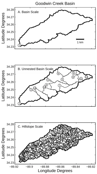
GCEW has a drainage area of 21.19 km2, and the rainfall– runoff data for the basin come from 13 stream gauges and 31 rain gauges (Blackmarr and the Channel and Watershed Processes Research Unit, 1995). For this study, we excluded another stream gauge in the basin (gauge 10) because of problems with its data. Figure 1 shows three maps of GCEW that represent basin, unnested basin, and hillslope scales. Map A shows only the drainage area of GCEW, defined here as the upstream area of stream gauge 1. Map B shows the drainage areas of the 13 stream gauges, which can overlap (e.g. gauges 4 and 7). Map C shows the drainage areas of 544 hillslopes that compose GCEW. Rainfall and stream-flow data were used to evaluateψfor the entire GCEW area (see Map A) and for each unnested sub-basin of GCEW (see Map B). Values ofψwere determined for numerous events, and the methods for selecting events, estimating total event rainfall and streamflow, and determiningψare given below.
3.1 Selecting rainfall–runoff events from streamflow
data
We selected rainfall–runoff events having moderately simple rainfall and streamflow conditions. Consecutive 2-day peri-ods from 1981 to 1995 were identified where records indicate that (1) rainfall occurred on the first day of the 2-day period at all rainfall stations, (2) streamflow was present in all gauged channels on both days, and (3) streamflow at gauge 1, the outlet of GCEW, had a single distinct peak. These 2-day pe-riods capture either an entire rainfall event or a subset of one
34.23 34.24 34.25 34.26 34.27 34.28
1
1 km
A. Basin Scale
Latitude Degrees
Goodwin Creek Basin
34.23 34.24 34.25 34.26 34.27 34.28
Latitude Degrees
1 2
3
4
5 6
7 8 9
11 12
13 14
B. Unnested Basin Scale
−89.92 −89.9 −89.88 −89.86 −89.84 −89.82
34.23 34.24 34.25 34.26 34.27 34.28
Longitude Degrees
Latitude Degrees
C. Hillslope Scale
Fig. 1. Decomposition of GCEW into three spatial scales. Plot A shows the basin scale (a= 21.19km2
) along with the location of stream gauge 1, the outlet of GCEW. Plot B shows the unnested basin scale (a/n= 1.63
km2
) and the locations of 13 stream gauges. Plot C shows the hillslope scale (a/m= 0.04km2
).
30
Fig. 1. Decomposition of GCEW into three spatial scales. Plot A
shows the basin scale (a=21.19 km2) along with the location of stream gauge 1, the outlet of GCEW. Plot B shows the unnested basin scale (a/n=1.63 km2) and the locations of 13 stream gauges. Plot C shows the hillslope scale (a/m=0.04 km2).
that lasts more than two days. In the latter case, it is possible that rainfall contributing to the outlet peak occurs prior to the 2-day period. Therefore, we used the time of peak streamflow at gauge 1,ti, as a reference time for an eventi. We selected
only those 2-day periods where (4) rainfall did not occur at any of the stations from 48 to 24 h beforeti, and (5) rainfall
did occur at all rainfall stations during the 24 h period leading up toti. A computer algorithm found 148 events that meet
criteria (1) to (5), about 10 events per year. For each event, step (4) requires that antecedent conditions include a 24 h period of zero rainfall. This step provides little constraint on antecedent soil moisture, which can be near zero in late sum-mer and near 1 in winter (Furey and Gupta, 2005).
3.2 Estimating rainfall and runoff for events
We generated rainfall fields using data from the 31 rain sta-tions in GCEW. Rain station data for the basin record accu-mulated rainfall depth per event, and the time interval be-tween data points is not a constant. Therefore, we first pro-duced a new 5-minute-interval time series of rainfall rates for each station by expressing accumulated rainfall values in terms of rain rate and then linearly interpolating between data points. We set interpolated rain rates that were nega-tive to zero. Then, for each event, we generated a time se-ries of rainfall fields beginning atti−dand ending atti+d,
whered is a 24 h time period. At each 5-minute time step, we produced a rainfall field by triangulating rain rates at the stations and then linearly interpolating between values; other more-involved approaches could be used that charac-terize rainfall fields better when rainfall spatial variability is high. For each event in this study, there are 576 five-minute fields (2 days×24 h day−1×12 five-minute fields h−1) that describe the space–time structure of rainfall, including 5-minute periods where there is no rain. Each field covers GCEW and can be partitioned into areas corresponding to the sub-basins (unnested or otherwise) and hillslopes in the basin.
Using stream gauge data, we estimated the runoff gener-ated during an eventifrom each basinj by subtracting base-flow as
˜
qi,j(t )=qi,j(t )−qi,j ; s1≤t≤s2, j=1,2, . . . ,13 (2) where
q
i,j =mint (qi,j(t )); (ti−d)≤t≤ti
s1=max(t )whereqi,j(t )=qi,j ; (ti−d)≤t≤ti
s2=min(t )whereqi,j(t )=qi,j; ti < t. (3)
Here,qi,j(t )represents observed streamflow andqi,j
repre-sents antecedent streamflow. We interpret q
i,j as baseflow
that is constant during an event and subtract it fromqi,j(t )to
obtain event runoff,q˜i,j(t ).
3.3 Determiningψ
We estimated runoff/loss ratios at the basin scale,ψi, and
unnested basin scale,ψi,j wherej=1,2, . . . ,13 denotes an
unnested basin. For the basin scale (Fig. 1, Map A), we used Eq. (1) where the variables for runoff/loss ratio, total rainfall, and streamflow are each given a subscripti. We averaged rainfall over the drainage area of stream gauge 1 at each time step to obtain rainfall rate, denotedri(t ), and used Eq. (2)
to estimate streamflow, denotedq˜i(t ). For the unnested basin
ψi,j =
ri,j
li,j
−1 ; ri,j = s2
Z
s1
ri,j(t )dt,
li,j =1/aj s2
Z
s1
ri,j(t )aj+
X
k∈Bj
˜
qi,k(t )− ˜qi,j(t )
dt, (4)
whereBjis a set of gauged sub-basins of basinj. IfBj is an
empty set, thenP
k∈Bjq˜i,k(t )=0.
For the unnested basin scale, we unnested data from a gauged basin j using data from a set Bj of gauged
sub-basins. Table 1 lists the 13 stream-gauged basins in GCEW (j=1,2, . . . ,13) and shows sub-basin gauges in set Bj, if
any, and drainage areas before and after unnesting. We ob-tained the unnested drainage area for basin j by subtract-ing the areas of the sub-basin gauges in Bj from the area
of basinj; e.g. for basinj =2, the unnested drainage area is a2=17.92−(8.78+3.57+1.24+1.63)=2.7 km2. We used CUENCAS (Mantilla and Gupta, 2005) to determine an unnested rainfall time series for eventiand basinj, de-notedri,j(t ), by averaging rainfall over the unnested area of
j at each time step. Finally, we evaluated the unnested total runoff for eventiand basinj as the difference between total runoff exiting and total runoff entering the unnested area.
3.4 Selecting a final collection of events
For many of the 148 events, there are unnested basins for which water balance is unresolved. This feature arises in two ways. For certain events, there is at least one unnested basin for which the runoff exiting its area is less than the runoff en-tering its area at upstream gauges. In Eq. (4), this situation means q˜i,j(t ) <Pk∈Bjq˜i,k(t ), which suggests that water
loss occurs within the river channels of unnested basinj. It is most often found with basinj =2, which coincidentally has the largest setBjof sub-basin gauges. Also, for some events,
there is an unnested basin for which the integrand in Eq. (4) is negative, meaningq˜i,j(t ) > ri,j(t )aj+Pk∈Bjq˜i,k(t ). This
situation suggests that there is an unknown source of wa-ter that contributes to runoff exiting unnested basinj. These two features could have natural or human-induced physical origins, but they also could originate from inaccuracies in streamflow measurements, rainfall estimates, and baseflow
q
i,j estimates.
We selected events for which water balance is resolved in a minimum of 11 unnested basins. This brings the num-ber of events to 112, still a large numnum-ber by which to de-velop and test a top-down model. These events were put into three groups: 112 events with 11 unnested basins (Case I), 75 events with 12 unnested basins (Case II), and 20 events with 13 unnested basins (Case III). Case I events include Case II events which include Case III events. We grouped the data to test our model. As explained in Sect. 4, our model predicts
Jan Apr Jul Oct Jan
0 10 20 30 40 50 60 70 80
Time Of Year l i
[mm]
A.
Jan Apr Jul Oct Jan
0 10 20 30 40 50
Time Of Year
Volumetric Soil Moisture (%)
B.
0 20 40 60 80 100
0 0.2 0.4 0.6 0.8 1
Case I: 112 Events 11 Obs. per Event
l
i,j [mm]
Non−Exceedance Probability
C.
Fig. 2. Plot A shows water-loss depths at the basin scale,li, for 112 events versus time-of-year. Plot B shows
volumetric soil moisture content versus time-of-year from Furey and Gupta (2005). Plot C shows empirical
CDFs of water-loss depths at the unnested basin scale, li,j, for 112 events. Each distribution represents a
rainfall-runoff event.
31
Fig. 2. Plot A shows water-loss depths at the basin scale,li, for 112
events versus time of year. Plot B shows volumetric soil moisture content versus time of year from Furey and Gupta (2005). Plot C shows empirical CDFs of water-loss depths at the unnested basin scale,li,j, for 112 events. Each distribution represents a rainfall–
runoff event.
similarity between rescaled cumulative distribution functions (CDFs). Statistical tests of this feature can be sensitive to the number of samples that comprise empirical CDFs. Thus, while Case I events include those for Case III, it is possible that differences between the cases in the number of samples per empirical CDF lead to contradictory test results that in-validate the model.
The process we used to select events was designed to pro-vide a large number of events but, as expected, it eliminated many events from analysis. Nonetheless, events for each case
Table 1. Properties of gauges used in this study.
ARS Basin ID Drainage area Sub-basin gauges Unnested drainage area gauge ID j
h
km2i SetBj aj
h
km2i
1 1 21.39 (a) 2 3.47
2 2 17.92 3, 4, 13, 14 2.70
3 3 8.78 5, 6 3.29
4 4 3.57 7 1.97
5 5 4.30 8, 9 2.57
6 6 1.19 – 1.19
7 7 1.60 – 1.60
8 8 1.55 11, 12 0.97
9 9 0.18 – 0.18
11 10 0.28 – 0.28
12 11 0.30 – 0.30
13 12 1.24 – 1.24
14 13 1.63 – 1.63
span a broad range of streamflow conditions. Among events, the smallest streamflow peaks at the outlet of GCEW are 0.21, 0.25, and 0.40 m3s−1 for Cases I to III, respectively. The largest streamflow peaks at the outlet of GCEW are 102, 47.8, and 43.7 m3s−1 for Cases I to III, respectively. The small events have return periods of less than 1 yr, while the large events have return periods of approximately 2 yr for Cases II and III and 5 yr for Case I. Both the event selec-tion process and the period of time we investigated, 15 yr, are responsible for the lack of events having return periods that exceed 5 yr.
3.5 Soil moisture in GCEW and a physical-statistical
hypothesis to test against the model
Before developing our model, we compared observations of water-loss depths at the basin scale,li, to historical
observa-tions of soil moisture in GCEW at the point scale. Figure 2a presents values ofliversus time of year for the Case I events.
Values are low from December to March and high from July to October. The peak water-loss depth for GCEW occurs around late August. Figure 2b comes from Furey and Gupta (2005) and shows observed values of volumetric soil mois-ture content taken 5 cm below soil surface at two point loca-tions in and near GCEW from January 1999 to June 2004. The general relationship betweenli and time is a mirror
im-age of the general relationship between soil moisture and time.
Spatial distributions of water-loss depth in GCEW also ap-pear to depend on soil moisture. Figure 2c shows the empir-ical CDFs of water-loss depth at the unnested basin scale,
li,j, for the 112 events. Each CDF consists of 11 values of
water-loss depth corresponding to 11 unnested basins. The figure shows that distributions that have a large mean tend to have a large variance and vice versa. Because a largeli,j
implies that soil moisture is low (dry), it suggests that the
spatial variability of soil moisture in GCEW is greatest when the spatial-mean soil moisture is low. This feature is consis-tent with soil moisture observations in other humid climate basins (Brocca et al., 2007). The patterns in Fig. 2 show that soil moisture plays an important role in runoff and loss in GCEW and should be a component of our model.
The observations presented in Fig. 2 also lead to a hypoth-esis, as follows. Plots A and B in Fig. 2 suggest that li is
roughly proportional to some function of 1/θ, whereθ de-notes point-scale soil moisture. It also suggests that thatli
characterizes surface infiltration amount as a first-order ef-fect in GCEW. Based on the observations, we infer thatli,j,k
for any hillslope within an unnested sub-basin is also propor-tional to some function of 1/θ; there are no data sets available to test this idea directly. Hydraulic conductivityK(θ )is ob-served to be proportional to a function ofθbecause, as soil moisture decreases, conductivity decreases (Brutsaert, 2005, p. 274–275, Figs. 8.23 and 8.25). A widely used parametric relationship for conductivity isK(θ )=Ksf (θ ), whereKsis hydraulic conductivity at saturation, andf denotes a func-tion ofθ(Brutsaert, 2005, p. 279-280). Spatially variableKs is commonly modeled as a lognormal random variable (e.g. Govindaraju et al., 2006; Meng et al., 2006), which implies thatK(θ )is lognormal within a hillslope. These relationships serve as the basis for a physical-statistical hypothesis: hills-lope water loss is inversely related to a function of a lognor-mal random variable. We show that our model supports this hypothesis at the end of Sect. 6.
4 Runoff–loss model
Such a model provides a method of using observations of
ψat the basin and unnested basin scales to estimate runoff generation and losses at the hillslope scale, where practically no observations are available. Our first step in developing the model was to explore the temporal and spatial variability of runoff/loss ratios at the unnested basin scale,ψi,j, for Case I
events. We wanted to determine if a simple rescaling ofψi,j
with respect to a measure of an overall event magnitude could account for event-to-event changes.
4.1 Establishing model form – temporal structure
Figure 3a shows the empirical CDFs ofψi,jfor Case I events.
There are 112 CDFs that correspond to 112 events, and each CDF consists of 11 unnested basins. For each event i, we evaluated the geometric mean of observed runoff/loss ra-tios, gi, and then rescaled the observed ratios as ψi,j/gi.
Figure 3b shows the CDFs of this rescaled runoff/loss ratio. The curves in Fig. 3b collapse nicely, indicating that tempo-ral variability can, to a first order, be accounted for by the use of the geometric mean as a simple scale parameter. An alter-native approach is to rescaleψi,j by the arithmetic mean, but
test results (not shown here) indicate that a weaker collapse occurs. Rescalingψi,j by its geometric mean is equivalent
to shifting log(ψi,j)by its arithmetic mean, i.e. computing
log(ψi,j)−log(gi). Thus, the results in Fig. 3 indicate that
an event-by-event first-moment shift yields similar distribu-tions.
We took a step further to see if there is improvement when incorporating second moments (variances). If the event-by-event variances are all the same, then the first-moment shift will suffice. Otherwise, we must take variances into consider-ation. We incorporated a second-moment correction by com-puting(log(ψi,j)−log(gi))/σˆi, whereσˆi is the standard
de-viation of log(ψi,j). Figure 3c shows the CDFs of the
expo-nential of this quantity, which is(ψi,j/gi)1/σˆi. The collapse
improves compared to that in Fig. 3b, indicating that rescal-ing should account for temporal differences in variances. The implication of the results presented in Fig. 3 is that event-to-event temporal variability in the spatial distribution ofψi,j
can be characterized quite well by the use of two parame-ters, the mean and variance of log(ψi,j). The results in Fig. 3
serve as the basis for developing our model.
4.2 Establishing model form – spatial structure
The model we develop needs to capture the features pre-sented in Fig. 3 but also connect runoff/loss ratios across scales in a way that respects their nested spatial correlation structure. At the unnested basin scale, we expect a high de-gree of spatial correlation among values ofψi,j for eventi
because they will be influenced by overall event magnitude. If we compare the spatial distribution ofψi,jfor a large event
to one for a small event, e.g. large vs. small rainfall amounts, then we expect that the two distributions will be distinct.
Fig. 3. Plot A shows a semi-log plot of empirical CDFs of runoff-loss ratios at the unnested basin scale,
ψ
i,j, for
112 events. Each distribution represents a rainfall-runoff event. Plot B shows corresponding CDFs of
ψ
i,j/g
i,
and Plot C shows corresponding CDFs of
(
ψ
i,j/g
i)
1/σˆi
.
32
Fig. 3. Plot A shows a semi-log plot of empirical CDFs of
runoff/loss ratios at the unnested basin scale,ψi,j, for 112 events.
Each distribution represents a rainfall–runoff event. Plot B shows corresponding CDFs ofψi,j/gi, and Plot C shows corresponding
CDFs of(ψi,j/gi)1/σˆi.
This effect can be modeled by takingψi,j to be a function
of ψi where the value of ψi reflects the overall event
ef-fect. Likewise, for unnested basinj, we can model hillslope runoff/loss ratios to be a function ofψi,j whereψi,j reflects
the overall event effect.
The nested structure of runoff/loss ratios must also be weighted by the drainage areas with which they are associ-ated. Suppose a basin is partitioned into five unnested basins,
j=1,2, . . . ,5, whereψi,1occupies 80 % of the total basin area while the remainingψi,joccupy 20 %. The dependency
ofψi,1on the overall event effect, represented byψi, will be
stronger than that of the remainingψi,j simply becauseψi,1 represents a larger fraction of the basin.
Discrete random cascade models (Gupta and Waymire, 1993) have a nested structure with spatial characteristics like those described above. Therefore, we can use the equations that define a cascade model to help establish the equations that define our model. A brief self-contained explanation of random cascades is given below that motivates the functional form of our model.
Consider a discrete random cascade spatial model with a branching numberb; i.e. a region of areaa0=1 is divided intob subregions of equal size (called level-1 subregions), each of these subregions is subdivided intobsubregions of equal size (called level-2 subregions), and so on. Denote to-tal mass in the whole region byM0, and denote mass in the jth level-1 subregion byM1,j,j=1, . . . , b. Then, under the
random cascade model,M1,j andM0are related by M1,j
d
=(1/b)W1,jM0, (5) where=d means “equality in distribution”, andW1,jare
inde-pendent and identically distributed (iid) level-1 cascade gen-erators with expectation 1. To understand the implications of this equation in terms of mean mass conservation, we can take the expectation of Eq. (5) to obtain
E[M1,j] =E[M0]/b. (6)
Therefore,E[M0] =bE[M1,j], showing that mass
conserva-tion holds in a mean sense. The area of a level-1 subregion is
a1,j=1/b, and we can take the logarithm of equation (5) to
obtain ln(M1,j)
d
=ln(M0)+ln(a1,j)+ln(W1,j). (7)
Here, total massM1,j depends onM0, whereM0reflects the overall mass, andM1,jdepends on the fraction of the overall
area. These relationships parallel those we want for a model ofψ. An expression like Eq. (7) can also be written for each level-nsubregion. For example, it can be modified to a re-lation between total mass for a level-2 subregion, with area 1/b2, and total mass M1,j. Finally, notice that Eq. (7)
in-volves a Markov-like property. In a Markov process, a able at the present time that is conditioned on a set of vari-ables representing past times has the same distribution as a variable that is conditioned on only the most recent past time (Feller, 1968). Random cascades have a Markov-like prop-erty because a given spatial scale influences only the next finer spatial scale (Over, 1995).
We can modelψ like a random cascade, though not ex-actly as one. A random cascade model leads to a limit mass distribution after a large number of subdivisions of space. It describes a process, e.g. rainfall, at a large number of spatial scales. By contrast, the smallest spatial scale for a model of
ψis the hillslope; physical reasons are given in Gupta et al. (2010). Also, cascades are random spatial measures that obey mass conservation in a mean sense, as shown by Eq. (6), but
ψdoes not obey this condition. Rather, it is the components ofψ(i.e. total rainfall and total loss) that obey mass conser-vation, as shown in Sect. 4.7.
In the sections that follow, we develop a runoff–loss model based on two equations that are each similar in form to Eq. (7), but are more general. Each equation characterizes how ψ at one spatial scale depends on bothψ at the next coarser spatial scale and drainage area fraction. We introduce the model in terms of random and then fixed unnested basins and hillslopes. Before testing the model, we also discuss how it connects to water balance.
4.3 Definition of model variables
We develop a model under the postulate that certain prop-erties ofψ observed at the basin scale are preserved down to the hillslope scale. Consider a basin of area a and di-vide it into n unnested basins of similar size and m hill-slopes of similar size where m > n. We letmj denote the
number of hillslopes in an unnested basinj such thatm=
Pn
j=1mj. We let aj denote the area of unnested basin j
wherej =1,2, . . . , n andaj,k denote the area of hillslope
kin unnested basinj wherek=1,2, . . . , mj. It follows that
a=Pn
j=1aj=Pnj=1
Pmj
k=1aj,k. Finally, we leta/ndefine the scale associated with the unnested basins anda/m de-fine the scale associated with the hillslopes. Thus, we con-sider three different spatial scales: basin scale a, unnested basin scalea/nwheren >1, and hillslope scalea/mwhere
m > n. Figure 1 shows the decomposition of GCEW into these scales.
Random variables Ri andLi express basin scale
condi-tions in the model; see Table 2. They represent total rainfall and total water loss for eventiin a basin, respectively. Real-izations are denoted byri andli. A given event is not
asso-ciated with a particular rainfall amount unlessri is specified.
Rather, a given event simply represents a distinct period of time where rainfall from a single storm produces runoff from a basin and streamflow conditions at the end of the time pe-riod are equal to those at the beginning.
Random variables J, aJ,Ri,J, and Li,J express spatial
variability at the unnested basin scale; see Table 2. Random variableJ represents the stream-gauged unnested basins in GCEW so that a realization,j, represents a specific unnested basin. Random variableaJ represents the drainage areas of
unnested basins so that a realizationaj represents the area
of a specific unnested basin. Random variablesRi,J andLi,J
Table 2. Variables that represent random and fixed locations (in space) for areaa, total rainfallR, total lossL, and runoff/loss ratioY. Realizations ofR,L, andY(not shown) are obtained using a lowercase letter; e.g. a realization ofRi,j is given byri,j.
Scale Location Area Total rainfall Total loss Runoff/loss ratio Basin Fixed a Ri Li Yi
Unnested basin Random aJ Ri,J Li,J Yi,J
Fixed aj Ri,j Li,j Yi,j
Hillslope Random aj,K Ri,j,K Li,j,K Yi,j,K
Fixed aj,k Ri,j,k Li,j,k Yi,j,k
at the unnested basin scale. Realizationsri,J andli,J refer to
an unnested basin with an outlet at a random location, while realizationsri,j andli,j pertain to a specific unnested basin,
j.
Random variablesK,aj,K,Ri,j,K, andLi,j,K represent
spatial variability at the hillslope scale, and their meanings parallel those for the unnested basin scale; see Table 2. Thus,
Krepresents the hillslopes in an unnested basin so that a re-alization,k, represents a specific hillslope. Random variable
aj,K represents the drainage areas of hillslopes in basinj,
and a realizationaj,krepresents the drainage area of a
spe-cific hillslope in unnested basinj. Lastly, random variables
Ri,j,K andLi,j,K represent total event rainfall and total
wa-ter loss for eventiin unnested basinj at the hillslope scale. Realizationsri,j,K andli,j,K refer to a hillslope at a random
location in unnested basinj, and realizationsri,j,kandli,j,k
refer to a hillslope at a given location in unnested basinj. Table 2 provides a comparison between the notations used to represent the basin, unnested basin, and hillslope scales. The connection between variables across scales has been made systematic. The first index corresponds to an event (time), the second index corresponds to the unnested basin scale (space), and the third index corresponds to the hillslope scale (space). Thus, the number of indices attached to a ran-dom variable defines its spatial scale. One index refers to an eventi at the basin scale, e.g.Li; two indices refers to an
eventiat the unnested basin scaleJ, e.g.Li,J; and three
in-dices refers to an eventifor a fixed unnested basinj at the hillslope scaleK, e.g.Li,j,K.
4.4 Model equations for random unnested basins and
hillslopes
The model equations introduced below represent a general-ization of the random cascade model given in Eq. (7). The nature of the generalization is explained after the model is introduced. Before introducing the equations, we make some assumptions about unnested basin and hillslope distributions. Assume that J has a uniform distribution on the integers 1, . . . , n, such that all unnested basins have the same prob-ability of being selected at random. This definition is consis-tent with our analysis of empirical CDFs in Sect. 4.1. Like-wise, assume thatK|J=j has a uniform distribution on the integers 1, . . . , mj, such that all hillslopes in unnested basinj
have the same probability of being selected at random. Also, assume thatJandKare independent of all random variables
RandL.
Let Yi=Ri/Li−1 be a random variable for the
runoff/loss ratio at the basin scale. Similarly, let Yi,J =
Ri,J/Li,J−1 andYi,j,K=Ri,j,K/Li,j,K−1 be random
vari-ables at the unnested basin and hillslope scales. For a random variableX, letG[X]denote the geometric mean ofX. Then, assume that for a given eventi
ln(Yi,J)=αi+βiln(Yi)+γiln(aJ/G[aJ])
+σiln(Ui,J) (8a)
ln(Yi,j,K)=αi,j+βi,jln(Yi,j)+γi,jln(aj,K/G[aj,K])
+σi,jln(Hi,j,K). (8b)
Equation (8a) describes the variability in runoff/loss ra-tios between unnested basins for eventi, while Eq. (8b) de-scribes the variability in runoff/loss ratios between hillslopes in unnested basinj for eventi. Here, in Eq. (8a),G[aJ]is
a geometric mean of unnested basin areas, ln(Ui,J)is a
ran-dom variable that has a mean of zero and is iid among events,
Yi is independent of ln(Ui,J), and parametersαi,βi,γi, and
σi can change from event to event because they depend oni.
The iid condition on ln(Ui,J)means that a common
probabil-ity distribution connects events. The subscriptiin ln(Ui,J)is
needed because realizations of ln(Ui,J|J=j )for one event
are not necessarily the same as those for another. Similarly, in Eq. (8b),G[aj,K]is a geometric mean of hillslope areas in
unnested basinj, ln(Hi,j,K)is a random variable that has a
mean of zero and is iid among events, Yi,j is independent
of ln(Hi,j,K), and parameters αi,j, βi,j,γi,j, and σi,j can
change from event to event because they depend oni. Equations (8a) and (8b) are general expressions of Eq. (7). Equation (8a) includes a random termUi,j that corresponds
to the cascade generatorW1,j. It also includes additional
pa-rameters,αi,βi,γi , andσi, and an additional subscript,i,
which accounts for changes from event to event. If values of
αi,βi,γiandσiare 0, 1, 1, and 1, then the resulting equation
looks like Eq. (7). However, values of these parameters are not specified a priori in the equation. Equation (8b) is also a general expression of Eq. (7) but only when it is modified to a relation between a level-2 subregion and a level-1 subregion. Later, in Sect. 4.6, we make an assumption that the distribu-tions of error terms for Eqs. (8a) and (8b) are the same, which
is essentially a scale invariance assumption. This assumption is found in random cascades whereWn,j is the same
dis-tribution for alln. Thus, taken together, Eqs. (8a) and (8b) are analogous to a “two-level” discrete cascade formulation where intermediate scales and scales finer than the hillslope scale are not explored. By including the event subscript i, Eqs. (8a) and (8b) comprise a space–time model rather than simply a spatial model. Over and Gupta (1996) considered a similar space–time extension of the random cascade model for space–time rainfall.
We next examine the physical implications of Eq. (8a) and then show how it explains the observations presented in Sect. 4.1. Equation (8a) characterizes runoff/loss ratios at the unnested basin scale. It captures two features that should be upheld, as described in Sect. 4.2. Namely, the equation shows that ln(Yi,J)depends on the runoff/loss ratio at the
next larger spatial scale,Yi, and only at this scale, a
Markov-like property. It also depends on unnested basin drainage area,aJ/G[aJ]. In the equation, the distributions ofaJ and
Ui,J do not change between events, and Ui,J accounts for
both spatial variability and “fixed event” temporal variabil-ity. The equation represents spatial variability through dif-ferences in drainage area, via aJ, and through differences
in physical conditions that affect water loss and runoff, via
Ui,J. For this paper, we interpretUi,J to represent the
influ-ence of antecedent soil moisture conditions for eventi. Tem-poral variability, as expressed byUi,J, is represented as an
ensemble where realizations ofUi,J change under repeated
occurrences of the same event.
Equation (8a) helps to explain the observations presented in Fig. 3 and discussed in Sect. 4.1. Taking the expectation of Eq. (8a), conditioned onYi=yi, gives
E[ln(Yi,J)|Yi =yi] =αi+βiln(yi)
+γi(E[ln(aJ)] −ln(G[aJ])) .
Because ln(G[X])=E[ln(X)]for any random variable X, the expression above can be rewritten as
ln(Gi(yi))=αi+βiln(yi) ; Gi(yi)=G[Yi,J|Yi=yi].
Here, E[ln(aJ)] −ln(G[aJ])=0 because ln(G[aJ])=
E[ln(aJ)], andGi(yi)corresponds to the sample estimates
of the geometric mean used to produce the CDFs in Fig. 3. Taking the exponential of both (ln(Yi,J)|Yi=yi), from
Eq. (8a), and ln(Gi(yi)), from the expression above, leads to
a rescaled runoff/loss ratio given as
Yi,J|Yi=yi
Gi(yi)
=
aJ
G[aJ]
γi Uσi
i,J,
or
Y
i,J|Yi=yi
Gi(yi)
1/σi
=
a
J
G[aJ]
γi/σi
Ui,J. (9)
Equation (9), in conjunction with our discussion in Sect. 4.1, indicates that distributions of ln(ψi,j/gi) can be
normal for each event but dissimilar between events be-cause of event-to-event changes inγi and/orσi;Ui,j cannot
be a source of dissimilarity because it is iid among events. In Sect. 4.1, we showed that CDFs of ψi,j collapse to a
common distribution when rescaling accounts for event-to-event changes in both Gi(yi) and σi (Fig. 3c). Based on
Eq. (9), this result occurs when aJ
G[aJ] γi/σi
is constant among events because aJ
G[aJ]=1,γi =0, orγi/σi>0 is
con-stant among events. In any case, only changes inGi(yi)and
σi are important for relating CDFs ofψi,j to a common
dis-tribution.
4.5 Model equations for fixed unnested basins
and hillslopes
Our objective is to develop an expression for the runoff/loss ratio at the hillslope scale that provides a method of simulat-ing event-based total runoff volume for each hillslope drain-ing an unnested basin. To meet this objective, we first need to describe ln(Yi,J)for a given unnested basinj and ln(Yi,j,K)
for a given hillslopekwithin unnested basinj. It is being as-sumed thatJ andKare independent of all random variables
Y. Also, subscript j forY means that we are conditioning on unnested basinj, and a subscriptkforY means that we are conditioning on hillslopek. Consequently,(Yi,j|Yi=yi)
is equivalent to (Yi,J|Yi=yi, J =j ),(Yi,j,k|Yi,j=yi,j)is
equivalent to(Yi,j,K|Yi,j=yi,j, K=k), and Eqs. (8a) and
(8b) provide the description we need when expressed con-ditionally as(ln(Yi,j)|Yi=yi)and(ln(Yi,j,k)|Yi,j=yi,j). In
these equations, unnested basin and hillslope drainage areas, respectively, are fixed. Because of this feature, we denote
aj0 =aj/G[aJ]
aj,k0 =aj,k/G[aj,K] (10)
as the area terms in the equations.
The expression obtained from Eq. (8a) for(ln(Yi,j)|Yi =
yi)describes the variability in runoff/loss ratios for a given
unnested basinj and eventi. The area term, a0j, expresses the relative contribution that the runoff/loss ratio for the unnested basin makes to the basin-wide value ln(yi). Ifaj0 =
1, then(ln(Yi,j)|Yi =yi)is independent of area. This
situa-tion can occur if all unnested basins have the same area, re-gardless of size. However, gauged unnested basins rarely, if ever, have the same unnested areas, including GCEW. When the unnested basin is given asj,Ui,J becomesUi,j. The
dis-tribution ofUi,j does not change between events, and, for a
given eventi,Ui,j accounts for both spatial variability and
fixed event temporal variability. The spatial variability de-scribed byUi,j represents an ensemble where realizations of
Ui,jchange under repeated copies of unnested basinj for the
same event. Differences in antecedent soil moisture between copies are postulated to represent this change.
Similarly, the expression obtained from Eq. (8b) for
hillslopekin unnested basinj and for eventi. Its area term,
aj,k0 , represents a relative contribution to ln(yi,j). Given a
hillslope,Hi,j,K becomesHi,j,k. The distribution ofHi,j,k
does not change between events, butHi,j,kaccounts for both
spatial variability and fixed event temporal variability. The rescaled runoff/loss ratio for a fixed basin is compara-ble to but significantly different from Eq. (9). From Eq. (8a), the expected runoff/loss ratio for a fixed basin is
E[ln(Yi,j)|Yi=yi] =αi+βiln(yi)+γiln(a0j),
which can be written as
ln(G˜i(yi, j ))=αi+βiln(yi)+γiln(a0j);
˜
Gi(yi, j )=G[Yi,j|Yi =yi],
because ln(G[X])=E[ln(X)]for any random variableX, as mentioned previously. Since G˜i(yi, j ) is given for a basin
j, it does not correspond to the sample estimates of the geometric mean used to produce the CDFs in Fig. 3. Tak-ing the exponential of(ln(Yi,j)|Yi=yi), from Eq. (8a), and
ln(G˜i(yi, j ))leads to a rescaled runoff/loss ratio for a fixed
basin given as
Yi,j|Yi=yi
˜
Gi(yi, j )
=Uσi
i,j
or
Y
i,j|Yi=yi
˜
Gi(yi, j )
1/σi
=Ui,j. (11)
Unlike Eq. (9), Eq. (11) shows that the distribution of
(Yi,j|Yi =yi), after a rescaling that includesσi, equalsUi,j
and thus is iid among events.
4.6 Assumptions for assigning water loss to hillslopes
To reach our final objective, we need to relateαi,j,βi,j, and
γi,j in Eq. (8b) toαi,βi, andγi in Eq. (8a) because
hills-lope observations needed to estimateαi,j,βi,j, andγi,j are
unavailable at present and are not expected to be available in the foreseeable future. Therefore, we let
¯
αi =1/n n
X
j=1
αi,j vα,i=1/n n
X
j=1
(αi,j− ¯αi)2, (12)
¯
βi =1/n n
X
j=1
βi,j vβ,i=1/n n
X
j=1
(βi,j− ¯βi)2,
¯
γi =1/n n
X
j=1
γi,j vγ ,i=1/n n
X
j=1
(γi,j− ¯γi)2,
whereα¯i is the average ofαi,j overj for eventi, and vα,i
is the variance ofαi,j over j for eventi. Likewise,β¯i and
¯
γi are averages andvβ,i andvγ ,i are variances. We assume
that, to a first order, vα,i=vβ,i=vγ ,i=0, which implies
thatα¯i=αi,j,β¯i=βi,j, andγ¯i=γi,j. We also assume that
¯
αi =αi, β¯i=βi, andγ¯i=γi, which means that αi,j=αi,
βi,j =βi, andγi,j =γi. We later assess the impact of these
assumptions by examining model results in the context of water balance. Substituting these last three relationships into Eq. (8b), conditioning onYi,j=yi,j andK=k, and
expo-nentiating the result gives
(Yi,j,k|Yi,j =yi,j)=exp(αi)yi,jβia 0 j,k
γiHσi,j
i,j,k.
In this expression, the right-hand side still depends on the hillslope scale, throughHi,j,kσi,j. To remove this dependence, we assume that the random variablesHi,j,kσi,j ,k=1,2, . . . , mj
are iid and
Uσi
i,j d
=Hi,j,kσi,j. (13)
This equation holds for eachkand gives
(Yi,j,k|Yi,j =yi,j) d
=exp(αi)yi,jβia0j,k γiUσi
i,j;
k=1,2, . . . , mj.
Now, (Yi,j,k|Yi,j =yi,j) is a function of variables at the
unnested basin and basin scales where observations exist. The distributions of(Yi,j|Yi=yi)and(Yi,j,k|Yi,j=yi,j)
must be specified to assign water loss to hillslopes. We as-sume that
(Yi,j|Yi=yi) d
=LN(µi,j, σi2) (14)
(Yi,j,k|Yi,j =yi,j) d
=LN(µi,j,k, σi2);
µi,j,k=ln(exp(αi)yi,jβiaj,k0
γi), (15)
where LN refers to a lognormal random variable and the dis-tribution parameters in parentheses denote the mean and vari-ance of the associated normal distribution. Here, normal dis-tribution variances are constant in space (among hillslopes and unnested basins). The assumption that distributions are lognormal requires that total rainfall exceeds total loss for a rain event; i.e. (Yi,j|Yi =yi) >0, (Yi,j,k|Yi,j =yi,j) >0,
and runoff occurs. It also requires that total rainfall is posi-tive. Under this assumption, we have
Ui,j d
=Hi,j,k
d
=LN(0,1) (16)
(Yi,j,k|Yi,j =yi,j)=d exp(αi)yi,jβia0j,k γiUσi
i,j,
indicating that(Yi,j,k|Yi,j=yi,j)is lognormally distributed
for a given event and unnested basin. The assumption also means thatσi,j =σi, whereσi =pVar(ln(Yi,j)|Yi=yi)and
σi,j=pVar(ln(Yi,j,k)|Yi,j=yi,j). Finally, the assumption
means that Eq. (8a), givenJ =j, and Eq. (8b), givenK=k, take the form of a linear regression model. Notice that the equality inσ’s follows from Eq. (13). It is a first-order ap-proximation and represents the simplest case of the expres-sion,σi,j=cσi. Given the difference in scale betweenσiand
σi,j, it is possible thatc >1.
Table 3. Results of thek-sample Kolmogorov–Smirnov (KS),k-sampleZc, and Lilliefors tests for(ψi,j/gi)1/σˆi.
Test H0– null hypothesis Do not rejectH0if . . . Case:result
k-sample KS Distributions are similar c <0.462 I:c=0.091 II:c=0.083 III:c=0.154
k-sampleZC Distributions are similar p >0.05 I:p=1.0
II:p=1.0 III:p=1.0
Lilliefors Distributions of the logarithm are normal l=0 I:l=0 for 90 events of 112 II:l=0 for 60 events of 75 III:l=0 for 17 events of 20
The observations given in Fig. 3b, which show that rescal-ingψi,j as(ψi,j/gi)1/σˆi leads to a collapse in distributions,
supports the assumption thatψi,j is lognormally distributed.
The physical basis of this feature is linked to the hypothesis explained in Sect. 3.5, where it is stated that the spatial distri-bution of saturated hydraulic conductivity, which influences soil moisture and thus water loss, is commonly found to be lognormal. As mentioned in Sect. 4.4, we interpretUi,J to
represent antecedent soil moisture conditions for eventi. A similar interpretation is made forUi,j andHi,j,kwhere fixed
event spatial variability arises through spatial changes in soil moisture.
If there is a need to generate total runoff at the hillslope scale for an observed rainfall event, then we need to make an assumption about the statistical connection between the runoff/loss ratio and total rainfall. We shall assume that the runoff/loss ratio and rainfall are statistically independent at both the unnested basin and hillslope scales; that is, the ran-dom variablesYi,j andYi,j,k are all independent of the
ran-dom variablesRi,j andRi,j,k. Thus, the model in Eq. (16)
for the runoff/loss ratio will remain the same if total rainfall at both scales is known and fixed.
Equation (16), together with the independence assumption in the previous paragraph, is the model that we set out to develop as it provides a way of assigning total water loss to hillslopes in three steps. First, we obtain values foryi,j
from observations ofψi,j at the unnested basin scale.
Sec-ond, based on Eq. (8a) when conditioned onJ=j, we ob-tain estimates ofαi,βi,γi, andσivia linear regression using
observations ofψi andψi,j and drainage areas of unnested
basins. Results from these two steps allow us to use Eq. (16) to generate realizationsyi,j,kfor each hillslopek. Third, we
determine values of total lossli,j,k=ri,j,k/(1+yi,j,k)given
that we have a realizationyi,j,kand an observation-based
es-timate ofri,j,k. An example is given below in Sect. 5.3.
4.7 Connection to water balance
We examined how the runoff–loss model is connected to wa-ter balance under the following simplified conditions. For eventi and basin j, let hillslope areaaj,k be the same for
allk, which means thataj,k0 =1 in Eq. (16). Water balance for unequal hillslope areas needs a more complicated formu-lation and is beyond the scope of this paper. Let the total rain-fall for eventibe known at the unnested basin and hillslope scales; that is,ri,j andri,j,kare fixed and nonrandom. Also,
let event i produce runoff, meaning that total rainfall over basinj exceeds total water loss orri,j> li,J andyi,J>0.
Under the conditions above, water balance for an event
i requires that (1) observed and modeled total runoff from basin j are equal and that (2) modeled totals of rainfall, runoff, and water loss in basin j equal the summation of corresponding hillslope totals, over allkhillslopes in basin
j. Requirement 1 must be satisfied on average because wa-ter loss is treated probabilistically. This situation is similar to mean mass conservation, which is used to construct canon-ical ensembles in statistcanon-ical mechanics and is central to the theory of random cascades, as illustrated in Sect. 4.2.
Requirement 2 is satisfied if
ri,j=1/mj mj X
k=1
ri,j,k, (17a)
li,j=1/mj mj X
k=1
E[Li,j,k|Li,j =li,j], (17b)
where (Li,j,k|Li,j =li,j)=(Li,j,K|Li,j=li,j, K=k).
These equations represent conservation of mass with respect to total rainfall depth and total depth of water loss. The condition under which Eq. (17b) holds is seen by noting that the definition of Yi,j,K gives Li,j,K=Ri,j,K/(Yi,j,K+1).
When rainfallri,j,k is fixed for allk, as shown in Eq. (17a),
we have Li,j,k=ri,j,k/(Yi,j,k+1) in Eq. (17b). Also, the
definition ofYi,j givesLi,j =Ri,j/(Yi,j+1). When rainfall
ri,j is fixed for allj, conditioning onLi,j =li,j, as shown
in Eq. (17b), is equivalent to conditioning on Yi,j =yi,j;
this feature follows becauseLi,j=Ri,j/(Yi,j+1)becomes
li,j =ri,j/(yi,j+1). Thus, with rainfall known at the
li,j=1/mj mj X
k=1 E
r
i,j,k
Yi,j,k+1
|Yi,j=yi,j
,
=1/mj mj X
k=1 E
"
ri,j,k
exp(αi)yi,jβiLN(0, σi2)+1
#
,
=ri,jE
"
1
exp(αi)yi,jβiLN(0, σi2)+1
#
.
Conservation of mass with respect to water loss holds when the expectation in the last equality equals 1/(yi,j+1).
This expectation takes the form ofE[1/(X+1)]withX log-normal, for which there is no analytical expression. In the limit asσi2→0 the expectation is given by 1/(exp(αi)yi,jβi+
1). Further, for smallσi, an asymptotic approximation
in-volving powers of σi can be made using standard
expan-sion techniques for integrals, but these results are beyond the scope of this paper. To honor conservation of mass in the small variance case, it is necessary forαi →0 andβi →
1 as σi2→0 so that, in the limit, the expectation equals 1/(yi,j+1). Observations presented in Sect. 5.1 show that
αi andβiare near these limits.
Conservation of mass with respect to runoff, a component of Requirement 2, follows from Eqs. (17a) and (17b). To see the logic of this connection, consider that randomness in hill-slope water-loss depth must lead to randomness in hillhill-slope and basin runoff. LetQi,j =(Qi,J|J=j )be a random
vari-able for the total volume of runoff for eventiand basinj. An observed value of runoff, a realization ofQi,j, is given as
qi,j = ri,j−li,jaj ; ri,j > li,j. (18)
Substituting Eqs. (17a) and (17b) into Eq. (18) gives
qi,j= 1/mj mj X
k=1
ri,j,k−1/mj mj X
k=1
E[Li,j,k|Li,j=li,j] !
aj
, (19)
=
mj X
k=1
(ri,j,k−E[Li,j,k|Li,j =li,j])aj,k,
=
mj X
k=1
E[Qi,j,k|Li,j =li,j].
This equation shows that the observed total basin runoff equals the summation of expected total runoff from hill-slopes, which supports Requirement 2, i.e. mean mass con-servation in terms of runoff. If Eqs. (17a) and (17b) hold true, then so does Eq. (19) and the runoff–loss model preserves water balance.
5 Analysis and results
5.1 Testing model relationships and assumptions
5.1.1 Equation (9): distributions of rescaled runoff/loss ratios at the unnested basin scale for random unnested basins
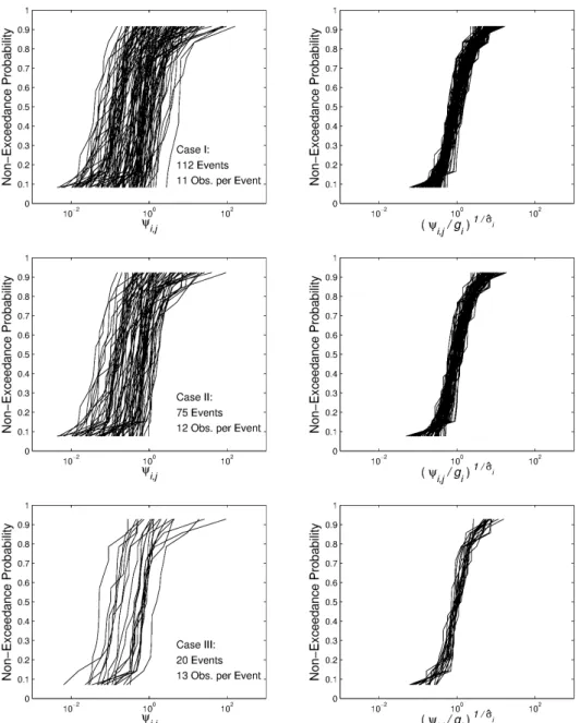
Figure 4 shows the empirical CDFs of runoff/loss ra-tios at the unnested basin scale, ψi,j, and the CDFs of
rescaled ratios given as(ψi,j/gi)1/σˆi, wheregiandσˆidenote
observation-based estimates ofGi(yi)andσi in Eq. (9). The
figure presents results for Cases I, II, and III. As explained in Sect. 3.4, the number of events and unnested basins for these cases are, respectively, (112,11), (75,12), and (20,13). The first case consists of the same events examined in Sect. 4.1. Results in the figure suggest, qualitatively, that rescaled ra-tios come from the same probability distribution.
Table 3 shows the results of comparing CDFs of rescaled ratios using thek-sample Kolmogorov–Smirnov test (Conover, 1999) and thek-sampleZC test (Zhang and Wu,
2007), which is shown to be more powerful. The first test re-quires that the number of points in each CDF is the same in the group of CDFs to be compared. Plots in Fig. 4 meet this requirement. Results indicate that rescaled distributions are statistically identical among all events.
Table 3 also shows the results of applying a Lilliefors test to the distribution of ln((ψi,j/gi)1/σˆi), the logarithm of
rescaled runoff/loss ratios, for each event. The Lilliefors test allows for both the mean and variance of ln(ψi,j)to change
from event to event, and thus it gives identical results when applied to(ψi,j/gi)1/σˆi, which is both mean- and
variance-corrected. Results in the table indicate whether a correction by the mean and variance yields identical distributions. For Case I events, they show that the hypothesis of normality is rejected at the 5 % level for 22 of the 112 CDFs. Some or all of the rejections could be erroneous, a type I error. Apply-ing the same tests usApply-ing a Bonferroni correction to account for the large number of individual tests (Hsu, 1996) indi-cates that all CDFs are normal except one. Similar results are found for Cases II and III.
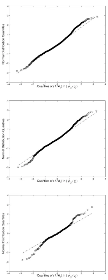
Figure 5 shows quantile–quantile (QQ) plots (Wilk and Gnanadesikan, 1968) for ln((ψi,j/gi)1/σˆi), representing the
logarithm of the rescaled ratios in Fig. 4. For each case, we grouped the ratios from all events to make a plot. The lines in the QQ plots for Cases I and II are relatively straight, sug-gesting normality or approximate normality among rescaled ratios; this linearity disappears if σi is not used to rescale
observations. Results for Case III deviate from normality. Based on Eq. (9) in Sect. 4.4, the deviations could mean that(γi/σi)ln
aJ
G[aJ]
varies among some or all events. Al-ternatively,(γi/σi)ln
aJ
G[aJ]
is constant among all events, but ln(Ui,J)is not iid among all events, as assumed. The
im-portant issue of lognormality is analyzed later in Sect. 5.1.3.
Fig. 4. Left: Semi-log plot of empirical CDFs of runoff-loss ratios at the unnested basin scale,ψi,j, for Cases
I to III. Each distribution represents a rainfall-runoff event. Right: Semi-log plot of corresponding CDFs of
rescaled runoff-loss ratios,(ψi,j/gi)1/σˆi.
33
Fig. 4. Left: Semi-log plot of empirical CDFs of runoff/loss ratios at the unnested basin scale,ψi,j, for Cases I to III. Each distribution
represents a rainfall–runoff event. Right: Semi-log plot of corresponding CDFs of rescaled runoff/loss ratios,(ψi,j/gi)1/σˆi.
5.1.2 Equation (8): relationship between runoff/loss ratios at the unnested basin and basin scales for fixed unnested basins
Equation (8) provides an expression for ln(Yi,j)for eventi
and unnested basin j, which takes the form of a multiple weighted linear regression model where there are two ex-planatory variables, ln(Yi)and ln(a0j), and a weight given
by 1/σi2. This model assumes that, on average, ln(Yi,j)
de-pends linearly on ln(Yi)and ln(aj0)for an event, but also
al-lows for the possibility that values of the coefficientsαi,βi,
andγi change among events. The model is not identifiable
if all three coefficientsαi,βi, andγi are allowed to change
with event; the problem that arises is similar to trying to fit a straight line to data where there is only one value for the explanatory variable. Thus, two of the three parameters must be fixed (no variation from event to event). In our analysis, we fixed the value ofβi =βandγi=γand treated the
inter-cept,αi, as a random variable (random from event to event).
The analysis also considered the influence that changes inσi
Fig. 5. QQ plot ofln((ψi,j/gi)1/σˆi), the rescaled runoff-loss ratios in Figure 4 after a log-transformation.
34
Fig. 5. QQ plot of ln((ψi,j/gi)1/σˆi), the rescaled runoff/loss ratios
in Fig. 4 after a log-transformation.
Results from the statistical analysis indicate that there is significant variability in the value ofαi between events for
Cases I and II but not Case III. For Case I, βˆ=1.027, ˆ
γ= −0.364, and the mean ofαiis estimated to be 0.316. The
variance ofαiamong events is estimated to be 0.009 and,
be-cause this value exceeds zero,αi changes between events as
assumed in our model. For Case II,βˆ=1.104,γˆ= −0.342, and the mean ofαi is estimated to be 0.449. The variance
of αi among events is estimated to be 0.002, and thus αi
changes between events. By contrast, results for the events in Case III indicate that the variance ofαiis not significantly
greater than zero, so that all theαiare equal to a single value
α. For Case III,βˆ=1.034,γˆ= −0.415, andαˆ=0.185. The left-hand column of Fig. 6 shows that observations of ln(ψi,j)and ln(ψi)for Cases I to III are, on average, linearly
related across events. The lines presented in the plots illus-trate the influence ofαion this relationship. To plot the lines,
we used values ofαiandβi =βobtained from our statistical
analysis but assumedγiln(aj0)=0 so that, based on Eq. (8),
ln(ψi,j)depends only on ln(ψi)and a line can be plotted.
The bottom line in a plot represents the minimum value of
αi among events, while the top line represents the maximum
value ofαi.
The left-hand column of Fig. 7 presents the same results shown in Fig. 6 but using only events that pass the Lilliefors test. The reduced number of events can be found in Table 3. Comparing the left-hand columns of Figs. 6 and 7 reveals that many of the events removed include “extreme” values of
ψi,j. This result suggests that events where the distribution of
ln(Ui,j)is not Normal, according to the Lilliefors test, tend to
have extreme values. Non-normality could arise if there are correlations among observations during these events that are unaccounted for in the model, if ln(Ui,j)is not Normal due
to some unique physical conditions in the rainfall–runoff pro-cess, or if the model does not well represent extreme events. Alternatively, the extreme values may simply represent mea-surement errors.
We have applied Eq. (8) as a linear mixed-effects statis-tical model where randomness is treated separately for each event. A measure of goodness of fit, likeR2, can be diffi-cult to interpret for such a model (Nakagawa and Schielzeth, 2013) and is not provided in Figs. 6 and 7. However, if a simple linear model is applied across all events for each of the cases in the two figures, thenR2values are around 0.6. A comparable and possibly better goodness of fit can be ex-pected for a linear mixed-effects model. One indication that this situation holds is that the Akaike information criterion (Akaike, 1974) is slightly better when treating events indi-vidually (linear mixed effects) instead of collectively.
−4 −3.5 −3 −2.5 −2 −1.5 −1 −0.5 0 0.5 1 1.5 −6
−4 −2 0 2 4 6
Case I
αi = 0.14 to 0.63
βi = 1.06
ln(ψi )
ln(
ψi,j
)
−4 −3 −2 −1 0 1 2 3 4
−4 −3 −2 −1 0 1 2 3 4
Residual Quantiles
Normal Distribution Quantiles
−4 −3.5 −3 −2.5 −2 −1.5 −1 −0.5 0 0.5 1 1.5 −6
−4 −2 0 2 4 6
Case II
αi = 0.40 to 0.57
βi = 1.12
ln(ψi )
ln(
ψi,j
)
−4 −3 −2 −1 0 1 2 3 4
−4 −3 −2 −1 0 1 2 3 4
Residual Quantiles
Normal Distribution Quantiles
−4 −3.5 −3 −2.5 −2 −1.5 −1 −0.5 0 0.5 1 1.5 −6
−4 −2 0 2 4 6
Case III
αi = 0.19
βi = 1.04
ln(ψi )
ln(
ψi,j
)
−4 −3 −2 −1 0 1 2 3 4
−4 −3 −2 −1 0 1 2 3 4
Residual Quantiles
Normal Distribution Quantiles
Fig. 6. Left: Plot ofln(ψi,j)versusln(ψi)for Cases I to III. To plot the lines, we used values ofαi(intercept)
andβi=β(slope) obtained from our statistical analysis, but assumedγiln(a′j) = 0; see equation (8). The
bot-tom line in a plot represents the minimum value ofαiamong events while the top line represents the maximum
value ofαi. Right: QQ plot of residuals obtained from statistical analysis results.
35
Fig. 6. Left: Plot of ln(ψi,j)versus ln(ψi)for Cases I to III. To plot the lines, we used values ofαi(intercept) andβi=β(slope) obtained
from our statistical analysis, but assumedγiln(aj0)=0; see Eq. (8). The bottom line in a plot represents the minimum value ofαi among
events, while the top line represents the maximum value ofαi. Right: QQ plot of residuals obtained from statistical analysis results.
5.1.3 Equation (14): lognormality of runoff/loss ratios at the unnested basin scale for fixed unnested basins
We tested the assumption given by Eq. (14) that(Yi,j|Yi=
yi)is equal in distribution to a lognormal. For this test, we
compared the relationship between quantiles of a normal dis-tribution and those of residuals from the statistical analysis results described in Sect. 5.1.2. If Eq. (14) is correct, then the residuals are normally distributed as ln(U )−E[ln(U )]. The right-hand column of Fig. 7 presents this comparison in a QQ plot for Cases I to III and indicates that the distribu-tion of residuals is close to normality. This result supports
the lognormal assumption given by Eq. (14). By compari-son, the QQ plots in Figs. 5 and 6 are, overall, further from normality. Differences in QQ plots between the three figures underscore the importance of both the area term in the model and Lilliefors test results.