Cooperation for Sustainable Forest Management: An Empirical Differential Game Approach

Analysis

Cooperation for sustainable forest management: An empirical differential

game approach☆

Pablo Andrés-Domenech

, Guiomar Martín-Herrán

, Georges Zaccour

⁎

LEF, AgroParisTech and INRA, UMR356 Nancy, France b_{GERAD, Canada}

c

IMUVA, Instituto de Matemáticas, Universidad de Valladolid, Spain d

HEC Montréal, Canada

a b s t r a c t

a r t i c l e i n f o

Article history:

Received 22 September 2014 Received in revised form 9 June 2015 Accepted 15 June 2015

Available online xxxx

Keywords:

Deforestation Sustainable forest Dynamic games optimal control Time consistency Emissions

We model the role of the world's forests as a major carbon sink and consider the impact that forest depletion has on the accumulation of CO2in the atmosphere. Two types of agents are considered: forest owners who exploit the forest and draw economic revenues in the form of timber and agricultural use of deforested land; and a non-forest-owner group who pollutes and suffers the negative externality of having a decreasing for-est stock. We retrieve the cooperative solution for this game and show the cases in which cooperation en-ables a partial reduction in the negative externality. We analyze when it is jointly profitable to abate emissions, when it is profitable to reduce net deforestation, and when it is optimal to do both (abate and reduce net deforestation). Assuming that the players adopt the Nash bargaining solution to share the total dividend of cooperation, we determine the total amount that the non-forest owners have to transfer to forest owners. Next, we define a time-consistent payment schedule that allocates over time the total transfer.

© 2015 Elsevier B.V. All rights reserved.

1. Introduction

The world's forests cover nearly one-third of the Earth's surface, but are decreasing at an alarming rate, with an area equivalent to the size of Costa Rica being deforested every year (FAO, 2010). World deforestation has become an issue of great international envi-ronmental concern for a number of reasons:first, the world's forests have an ecological value as carbon sinks. Second, forests host much of the world's biodiversity. Third, forests protect land and water re-sources,_filter water, regulate water regimes and help prevent land erosion and desertification. Fourth, forests provide economic, socio-cultural, aesthetic and recreational services, etc. In this paper we concentrate mainly on the role of forests as carbon sinks, even if the framework used here could be extended to include the other aspects.

We view forests as providers of competing economic and environ-mental goods. While forest logging brings economic revenues from both timber and agriculture on deforested land in the short run (FAO,

2006), excessive logging can exacerbate the problem of greenhouse gases (GHGs) accumulating in the long run. Reducing emissions from deforestation and degradation (REDD) has been put forward as a poten-tially cost-effective strategy to mitigate climate change. We build a model that accounts for GHG accumulation in the atmosphere in terms of anthropogenic emissions and carbon sequestration by the world's forests. The framework used allows one to: (i) evaluate the im-pact that forest depletion has on atmospheric GHG accumulation through the so-calledreduced-carbon-sequestration effect, which states that a tree that is cut cannot grow and hence cannot sequester carbon; and (ii) compare the short-term rewards of high emissions and inten-sive deforestation policies with their long-term costs due to excesinten-sive GHG accumulation and forest depletion.

There is a significant dynamic-games literature dealing with the role of excessive GHG accumulation (see, e.g., the early papers ofvan der

Ploeg and de Zeeuw (1992),Long (1992),Dockner and Long (1993)

and the literature review byJørgensen et al. (2010)). In this literature, emissions are a control variable and the issue is to determine the opti-mal emissions rate so as to reduce the environmental damage coming from the excessive accumulation of GHGs. Typically, these models con-centrate on the difficulty of coordinating optimal emission levels and treat carbon sequestration as exogenously given. That is, as a constant fraction of the total stock of greenhouse gases. In this paper we model total carbon sequestration by forests explicitly and endogenously. If for-ests worldwide become rarer as a consequence of agents' decisions then ☆ The second author's research is partially supported by MEC under projects,

ECO2011-24352, and ECO2014-52343-P, co-financed by FEDER funds, and COST Action IS1104. The third author's research is supported by NSERC, Canada.

⁎ Corresponding author at: HEC Montréal, Canada.

E-mail addresses:[email protected](P. Andrés-Domenech),

[email protected](G. Martín-Herrán),[email protected](G. Zaccour).

http://dx.doi.org/10.1016/j.ecolecon.2015.06.016

0921-8009/© 2015 Elsevier B.V. All rights reserved.

Contents lists available atScienceDirect

Ecological Economics

the ability of worldwide forests to sequester carbon is reduced. Afirst contribution of this paper to this literature is in explicitly accounting for the role of forests as a carbon sink instead of just using an exogenous component that will yield the same amount of tons of carbon seques-tered regardless of the state of the forests worldwide.

There is also a literature that deals with forest depletion using a dynamic-game approach (e.g.,van Soest and Lensink (2000),Fredj et al.

(2004, 2006),Martín-Herrán and Tidball (2005)andMartín-Herrán

et al. (2006)). In these articles the players are forest owners, who exploit their asset to obtain economic revenues; and a donor community, or an environmentally aware player, who is willing to compensate forest owners who engage in preservation efforts of the resource.

We develop in this paper a model that merges these two strands of the literature. On the one hand, forest owners exploit (and eventually deplete) the forest. Their actions have an environmental impact on the atmospheric accumulation of GHGs. On the other hand, the non-forest-owner group derives utility from production (i.e., emissions) and disutility from the accumulation of GHGs in the atmosphere. In this setting, it is this disutility they experience that may eventually turn them into donors to preserve the forest as a carbon sink. This modeling framework allows us to capture both the high opportunity cost of reducing deforestation and the negative economic externality that forest owners inflict on non-owners as a consequence of their de-forestation policy. Unlike the other aforementioned papers, we do not focus solely on forest conservation but also on its impact on GHG accu-mulation. In this sense, non-forest owners are also to decide on the best way to adjust their emissions.

The parameters of the model are empirically estimated, a rarity in the literature applying game theory to environmental problems. We be-lieve that this constitutes a valuable contribution to the literature and an interesting demonstration case for policy and decision makers on how strategic interactions affect the evolution of both GHG accumulation and forest depletion. We determine the jointly optimal outcomes and compare them to the non-cooperative or business-as-usual counter-parts. When the planning horizon is sufficiently long, then the coopera-tive solution is overall welfare improving. Cooperation partly reduces the negative externality and we analyze when it is profitable to abate emissions, when it is profitable to reduce net deforestation, and when it is optimal to do both (abate and reduce net deforestation). The results obtained show that it is preferable (cheaper) to invest in deforestation reduction rather than in emissions abatement when the perceived dam-ages are low. However, as the environmental damdam-ages increase, it be-comes optimal to combine emissions abatement with deforestation reduction.

Another aspect of key importance within the REDD literature is de-termining how these measures (i.e., measures involving emissions re-ductions) are to be implemented. In this paper we focus on the technical aspects related to thefinancial implementation of such poli-cies within a dynamic setting: The cooperative solution brings economic gains, however these are asymmetric: the non-owner group gains while forest owners lose. Thus any environmental agreement attempting to implement the cooperative solution will require monetary compensa-tion from the agents who win (non-owners) to the agents who lose (forest owners). Necessarily, forest owners have to be compensated with an amount at least equal to the difference between the sum of their intertemporal cooperative and non-cooperative payoffs. This com-pensation can be viewed as a payment for environmental services (PES) provided by forest owners. However, this requirement is not enough: When designing an intertemporal compensation mechanism (i.e., PES scheme), it is of key importance to allocate the transfers in such a way that no player has an economic incentive to deviate from the coopera-tive agreement at any instant of time, i.e., that the agreement be time consistent. We show that a division of joint payoffs using a dynamic Nash-Bargaining Scheme yields time-consistent outcomes.

The remainder of the paper is organized as follows: the model used for the two types of agents is presented inSection 2. InSection 3, the

non-cooperative optimal policies for each player are obtained. Then, in Section 4, we compute the optimal cooperative policies and compare them to their non-cooperative counterparts.Section 5is devoted to an-alyzing the feasibility and dynamic stability of the cooperative solution. Finally, all the results obtained are summarized inSection 6. The proofs are collected in the Appendices (Supplementary Material).

2. The Model

We consider two types of agents: forest owners and non-owners. Forest owners are modeled here as environmentally unconcerned agents who only care about revenues from deforestation, that is, they do not consider the consequences of their deforestation policy on GHG accumulation. Conversely, non-owners get revenues from the produc-tion of economic goods.1_{Their productive activity generates emissions} and this non-forest-owner group does take into account the negative ef-fects of their current emissions policies on GHG accumulation in the at-mosphere. This way of modeling allows us to capture the negative externality that forest owners create on the non-forest-owner group through the so-calledreduced-carbon-sequestration effect.

We wish to state from the outset that our assumption that forest owners are environmentally unconcerned agents is undoubtedly a sim-plifying one. Still, it can be motivated on at least two relevant grounds, namely, methodology and realism. First, this assumption allows us to compute the upper-bound monetary compensation that is needed to in-duce forestry countries to save their forests. Accounting for any addi-tional benefits of forests to their owners would decrease this value accordingly. Second, following many others, it has been argued by

Masoudi and Zaccour (2013)that“compared to other pressing

econom-ic issues, such as eradeconom-icating extreme poverty, offering essential serveconom-ices to their citizens (education, health care, etc.) and building infrastruc-ture, the environment is seen as a luxury service that developing countries cannot really afford in the short term.”Considering that defor-estation is mainly occurring in developing forestry countries, then our assumption reflects, albeit in a drastic way, this state of affairs.

2.1. The Forest Owners' Problem

Forest owners maximize their discounted stream of net revenues, which depend on their afforestation and deforestation rates,A(t) and D(t) respectively, as well as on the existing forest surface areaF(t) mea-sured in hectares. Net revenues are discounted at raterthroughout a finite-time horizon, denotedT. In the next section, we let the planning horizon vary and show how the optimization results depend on the value ofT.

Net revenues include gross revenuesR(t), afforestation costsκ1A(t) and deforestation costsκ2D(t), whereκ1andκ2are respectively the per-hectare afforestation and deforestation costs. The forest owners' ob-jective is the following:

max

A tð Þ;D tð Þ ZT

0

e−rt_{R tð Þ−κ}

1A tð Þ−κ2D tð Þ

½ dt; ð1Þ

whereA(t)∈[0,Amax] andD(t)∈[0,Dmax]. The upper bounds for affor-estation (Amax) and deforaffor-estation (Dmax) reflect the idea that there is a physical limit, in the short term, to afforestation and that deforestation is subject to a regulation that allows for it within certain limits. The value ofDmaxis set tofit the observed world deforestationfigures

1

provided by theFAO (2006). The definitions of all parameters, their values and their sources are provided in Appendix A.

We assume that the evolution over time of the forest area can be well approximated by the following linear differential equation:

F ð Þ ¼t A tð Þ þηF tð Þ−D tð Þ; F≥F≥0; Fð Þ ¼0 F0; ð2Þ

whereηis a positive parameter,Fis the maximum surface suitable to forest colonization andF0is the initial forest world's surface area in 2005 (FAO, 2006), i.e., nearly 4 billion ha. Eq.(2)is an extension of

van Soest and Lensink (2000)andFredj et al. (2006), whereA=η=

0 in thefirst andA= 0 in the second. Note that the linear specification in Eq.(2)approximates reasonably well forest expansion within a large interval around the current world forest areaF(0).

Forest owners obtain revenues from selling timber and agricultural products. Denote byq(t) the quantity of timber put on the market at timet, and let the pricep(t) be given by the following inverse demand function:

p tð Þ ¼p−θq tð Þ; ð3Þ

wherepis the choke price that sets demand equal to zero, andθits slope. The values of parameterspandθhave been calibrated using data given by FAO on timber prices and quantities.

The quantityq(t) comes from two different sources, namely, clear-felling and selective logging, and is given by

q tð Þ ¼yD tð Þ þyγδF tð Þ; ð4Þ

whereyD(t) is the amount of wood retrieved from clear-felling an area D(t) and the productyγδF(t) stands for the total selective-logging yield, which is lower (in per-hectare terms) than the yield obtained through clear-felling. Parameterydenotes the per-hectare timber yield and is typically measured in stems per hectare or cubic meters of timber per hectare.FAO (2006)provides an estimate for this parameter. Clear-felling an areaD(t) reduces the total forest size by the same amount. However, unlike deforestation, selective logging is assumed to have no impact on total forest land. According to FAO,“[selective logging]…is not necessarily destructive and can be done with low impact on the remain-ing forests, if the proper techniques are applied”.2_{Clearly, for selective} log-ging to have a negligible environmental impact, its per-hectare yield per unit of area must be much lower than the clear-felling one. This lower yield is accounted for by parameterγ(γb b1). Finally, according to FAO (2006), roughly one-third of the world's forests are used primarily for the production of wood and non-wood forest products. Parameter_δ takes into account the fact that only a fraction of the world's forests are actually being exploited.3

Agriculture revenues are equal to the prices times the yields of the different crops grown. For simplicity, we suppose that forest owners grow a single agricultural good, which we model as a composite good made of four representative crops that are commonly related to defores-tation processes. This good is sold in international markets at a given pricepA.4The total yield at timetdepends on the size of the available (previously deforested) land, given byF−FðtÞ, whereFstands for the maximum size or carrying capacity of the forest, and on the soil produc-tivityx(t).

Putting together the revenues from timber sales and agricultural products, we get the following expression for gross revenue:

R tð Þ ¼p tð Þq tð Þ þpAx tð Þ F−F tð Þ

: ð5Þ

As in Andrés-Domenech et al. (2011)—see also van Soest and

Lensink (2000)for a simpler version—we modelx(t) as follows:

x tð Þ ¼xþαð ÞtD tð Þ−βF−F tð Þ

F : ð6Þ

The above expression of the total productivity of landx(t) is the sum of three terms. Thefirst is a constant productivity termxthat measures the average yield in tons of crop per hectare of land for a representative agricultural good. The second term,α(t)D(t), captures the idea that newly deforested landD(t) is more productive. Variableα(t) measures the increase in thetotalaverage per-hectare production resulting from

deforesting an areaD(t). The third term,−βF−FðtÞ

F , accounts for the

pos-itive externality that forests generate on nearby agricultural land. For-ests are seen as a source of rain and a protective element for agricultural land. Parameterβmeasures the decrease (increase) in soil quality and, therefore, in agricultural productivity caused by forest de-pletion (expansion). The productivity increase of newly deforested land is given by

αð Þ ¼t ψx

F−F tð Þ: ð7Þ

Newly deforested land is more productive and parameterψ mea-sures the factor by which productivity is increased. However, this extra productivity needs to be normalized for all agricultural land. We divide the extra yield,ψx, by the total agricultural surface area,F−FðtÞ, otherwise the termα(t)D(t) in Eq.(6)would overestimate the real im-pact that deforesting an areaD(t) has.5

To recapitulate, forest owners maximize their net discounted eco-nomic revenues Eq.(1)with respect to their deforestation and affores-tation efforts,D(t) andA(t), respectively, and subject to the forest dynamics in Eq.(2).

2.2. The Non-owners' Problem

Non-owners optimize a two-part objective function. Thefirst part consists of a short-run gain derived from producing and consuming eco-nomic goods. The production of these goods generates pollution as a by-product and this pollution affects their utility. For simplicity, we sup-pose that the carbon intensity of the economy is constant. Hence,ceteris paribus, producing more goods is equivalent to emitting more.6_The sec-ond term in the objective of the non-forest-owner group represents an economic loss or damage related to the accumulation of emissions in the atmosphere. We will specify the functional forms of these two terms after describing the dynamics of the GHGs emissions and the stock of pollution.

Denote byE(t) the GHGs emissions by the non-forest-owner group. Emissions, in our model, are assumed to be exclusively anthropogenic and are given entirely by the emissions of the non-forest-owner group. By this we do not mean that forest owners do not emit but rather that their contribution to global emissions is negligible.7_{The dynamics} of the emissions rateE(t) is then given by

Eð Þ ¼t V tð ÞE tð Þ; E tð Þ≥0; Eð Þ ¼0 E0: ð8Þ

2 _{Source:http://www.fao.org/forestry/news/48681/en/.}

3 _{Invan Soest and Lensink (2000), the parametersγandδare set equal to one. Here we}

follow the more general specification used byAndrés-Domenech et al. (2011).

4

The pricepAis constant, unlikep(t), due to the fact that agricultural production on deforested land represents only a fraction of the world's total agricultural land.

5 _{Agricultural revenues are obtained by multiplying the productivity(6)by total}

agri-cultural land. Hence Eq.(6)has to account for averageper-hectareproductivity measured in tons of crop per hectare. For this reason, the termα(t)D(t) cannot be understood as the extra productivity of newly deforested land, but rather as the normalized productivity in-crease thatnewlydeforested land has ontotalagricultural land.

6 _{One could think of a more refined formulation, where the economy's carbon intensity}

can adjust, and where production increases can be compatible with constant emissions levels or even decreases.

7

The dynamics of emissions in Eq.(8)can also be written in a more familiar way, that is,

E ð Þt E tð Þ¼V tð Þ;

whereV(t) denotes the instantaneous speed of emissions variation, which is the non-owners control variable. Non-owners maximize their payoffs by adjusting their emissions, and their decision has an impact on the state of the system. For the sake of realismV(t) has been modeled as a bounded control variable (i.e.,Vmin≤V(t)≤Vmax), withVminb0 and VmaxN0. In the literature, it is more common to see emissions as aflow variable. Our modeling of emissions allows us to better account for the inertia of the productive and economic systems. Indeed, emissions take time to adjust and the upper and lower bounds onV(t) simply re-flect this idea that emissions cannot be increased or decreased at what-ever rate. One can think of these bounds as being given by the existence of technical, economic and/or political constraints.

The evolution of the stock of greenhouse gases in the atmosphere depends on emissions and on carbon sequestration by the world's for-ests and oceans. Forfor-ests worldwide sequester carbon as they grow, and according to theIPCC (2000)andFAO (2006), approximately half of the dry weight of forest biomass is carbon. To model carbon seques-tration by forests, one could measure the variation in the total forest biomass; however, this would present two main difficulties. First, the variation in total carbon biomass is difficult to measure. And second, measuring carbon sequestration through the variation in forest biomass underestimates the total carbon sequestration since timber captures are neglected. To overcome this problem, we make the simplifying assump-tion that forest owners manage a representative forest whose trees grow_—volume wise_—at an average and constant rate. Having a repre-sentative forest whose growth rate is constant allows us to express car-bon sequestration as a linear function of forest area alone (i.e., carcar-bon sequestered per hectare of forest land and per unit of time). The advan-tage of having carbon sequestration in terms of forest area rather than in terms of biomass variation is that one can easily consider timber cap-tures, while gaining a tractable and understandable way to measure car-bon sequestration.

Further, note that by measuring carbon sequestration as a function of the forests' surface area, one can account for the so called reduced-carbon sequestration effect, which is based on the simple principle that a tree that is cut cannot grow (i.e., cannot sequester carbon). Thus, it is straightforward to see that deforestation has a negative impact on carbon sequestration due to the reduction in forest area that it induces. Expression(9)below captures the dynamics of the atmospheric con-centration of carbon in terms of the forest stock, where parameterϕ re-flects the amount of carbon sequestered per hectare of forest and per unit of time.

We also consider the oceans as a second type of carbon sink. Denot-ed byS(t) the stock of GHGs (e.g., stock of CO2) in the atmosphere and byW(t) the amount of carbon that the oceans sequester at a given timet. The carbon uptake by the oceans has remained relatively stable during the last few years, and for this reason,Whas been assumed con-stant for simplicity's sake even if there exist small year-to-year varia-tions due to El Niño effects (Le Quéré et al. (2009)). The evolution of the stock of pollution is then given by the following differential equation:

Sð Þ ¼t E tð Þ−ϕF tð Þ−W; S tð Þ≥0; Sð Þ ¼0 S0: ð9Þ

Once the time evolution of the emissions rate and the stock of pollution have been described, we come back to the description of the non-owners' two-part objective function. Thefirst part concerns the payoff generated in terms of goods production and is described

by the concave increasing functionG(E). We adopt the following functional form:

G E tð ð ÞÞ ¼aE tð Þ−₂1bE2_{ð Þt; ð10Þ}

where parametersaandbare positive and have beenfixed in order to ensure thatG′(E)N0 for the relevant range of emissions. This spec-ification is similar to the one proposed in, e.g.,Dockner and Long

(1993)andBreton et al. (2005), with the only difference being that

we have included parameterbto calibrateG(E(t)) at the current world-level GDP.

The second term in the objective of the non-forest-owner group rep-resents an economic loss or damage related to the accumulation of emissions in the atmosphere. According to theIPCC (2007), increases in the atmospheric concentration of GHGs result in seawater levels ris-ing, temperatures increasing and seawater acidification. These process-es are all related to economic and environmental damage. We assume that the damage cost is given by a strictly convex and increasing func-tionL(S), withSthe stock of GHGs (e.g., stock of CO2) in the atmosphere. Although we acknowledge the existence of thresholds, extreme events and jumps in the damage,8our formulation, which is very common in the literature (see, e.g.,Benchekroun and Long (2002),Dockner and

Long (1993), van der Ploeg and De Zeeuw (1992), Breton et al.

(2006)), smooths the impacts of such phenomena rather than dealing with them explicitly. Needless to say, accounting properly for non line-arities and threshold effects in the damage cost would lead to a model of much greater complexity.

That being said, for a speci_fic function to qualify as a good candidate to model such damages we can think of yet another necessary require-ment: greenhouse gases, and most particularly CO2, have always been present in the atmosphere and represent a basic element for the exis-tence and development of life (e.g., plants). It is clear that it is not the presence, but the excessive accumulation of atmospheric GHGs that poses the problem. We adopt the following specification ofL(S) to cap-ture all these elements in a simple way:

L S tð ð ÞÞ ¼c S tð ð Þ−SÞ2

; ð11Þ

whereSis a natural threshold, beyond which the GHG concentration is considered excessive and economic and environmental damages are perceived. In practical terms, choosing a reasonable value forS—given the above speci_fication_—amounts to choosing a level of atmospheric GHGs for which there is no perceived damage. We identifySwith the pre-industrial level of GHGs (see, e.g.,Bahn et al. (2008)).

Taking into account the gain functionG(E) and the damage function L(S), we obtain the following objective functional, which is maximized by the non-forest-owner group:

ZT

0

e−rt½G E tð ð ÞÞ−L S tðð ÞÞdt−ϕðS Tð ÞÞe−rT; ð12Þ

whereris the market discount rate (the same as for forest owners), and ϕ(S(T)) is a salvage value.

Non-owners are modeled as forward-looking agents who consider the long-term impact of their decisions. The stock of emissions accumu-lates slowly and then has a long-term impact on non-owners' payoffs. Therefore, it is sensible to have a scrap-value function somehow related to the stock of emissions at the terminal date of the planning horizon. Such a salvage-value function can be generically written asϕ(S(T)). It is reasonable to think that, whatever the GHG stock at the terminal date, it will strongly impact future payoffs due to the long-term

8_{For instance, a small increase in the atmospheric concentration of GHGs can bring a}

persistence of greenhouse gases in the atmosphere. One could think of a more sophisticated scrap-value function that also depends on thefinal forest stock or on the emissions policy followed after the terminal date, or even define the scrap-value function as an identical problem to the one presented above in Eq.(12). Because we want to keep the model parsimonious, and because we want to be able to say something that is irrespective of what policies are chosen after the terminal date, we have chosen the following formulation forφ(S(T)), which depends on the terminal stock of greenhouse gases alone:

ϕðS Tð ÞÞ ¼ Z2T

T

e−r sð−TÞ_{L S Tðð ÞÞds: ð13Þ}

Although the salvage function in Eq.(13)is simple, it satisfies the fol-lowing desirable requirements: (i) it re_flects the idea that the terminal stock of GHGs matters and has an impact on future payoffs; (ii) it is easy to compute and does not depend on (potentially) unknown future policies; (iii) it keeps discounting in a natural way the cost of future en-vironmental damages; and (iv) the time span considered for the scrap value function is related to the planning horizon. In fact, if the planning horizon chosen is short, then the weight given for future environmental damages will likely be small as well and vice versa.

To wrap up, non-owners maximize their payoff in Eq.(12)adjusting the instantaneous variation of emissionsV(t), subject to Eqs.(8) and (9) and given the fact that the solution to Eq.(2)is inherited from the forest owners' problem.

3. Individual Optimization

In this section we characterize the optimal strategies of the two players when they act independently. As the forest owners' payoffs do not depend on emissions or on GHG accumulation, their payoffs are in-dependent of the action of non-owners. On the other hand, non-owners' payoffs are affected by the forest owners' decisions through the evolu-tion of the forest stock. In this setting, where there is a one-way interac-tion, Nash and Stackelberg equilibria coincide. Further, open-loop and feedback-information structures yield the same result. Given this, we canfirst solve the economic problem of the forest owners, and next, op-timize for the non-forest-owner group, taking the evolution in the forest stock as given.

In the rest of the paper we useOto denote the forest owners and⊖ to refer to the non-owners.

3.1. Forest Owners

Forest owners maximize their revenues in Eq. (1) subject to

Eqs.(2)–(5). The following proposition provides the optimal solution

to their control problem (the superscript nc stands for non-cooperation).

Proposition 1.For the parameter domain defined in Appendix A, the opti-mal control, state and co-state variables are given by9

Ancð Þ ¼t 0; Dncð Þ ¼t Dmax f or all t∈½0;T;

F tð Þ ¼ F0−

Dmax η

eηt_þDmax η ;

ð14Þ

λð Þ ¼t 1

η−r 1−eη−

r ð ÞðT−tÞ

h i

ð2θyDmax−pÞyγδþpAðx−2βÞ þ2F tð Þ θy2γ2δ

2_þ

pAβ

1 F

: ð15Þ

Proof. See Appendix B.■

The results show that the forest owners' optimal strategy con-sists in deforesting at maximum admissible level and not afforesting at all. As the problem is linear in the afforestation effort, and affor-estation is a pure cost in our setting, then the optimal strategy is ob-viously to setA(t) at its lowest admissible value, i.e.,A(t) = 0. Further, the marginal revenue from agricultural activity is positive for all admissible values ofD(t), includingDmax. Therefore, there is an incentive to deforest at the maximum level.10These results fol-low from the fact that, for our parameter domain, we have λ(t)≤0, for allt. Indeed: (i) the term 1

η−r½1−eðη−

rÞðT−tÞ_{is always}

neg-ative since 1

η−rand [1−e(η− r)(T−t)

] are of opposite sign, regardless of the values ofηandr; and (ii)ð2θyDðtÞ−pÞyγδþpAðx−2βÞN0, for

all admissible values ofD(t), includingDmax. Deforestation is mainly driven by the revenues obtained from growing agricultural prod-ucts on deforested land, rather than by the timber revenues that arise from deforestation itself. This is in line with other studies, e.g.,Barbier and Rauscher (1994),Barbier and Burgess (2001)and FAO (2006), which suggested that deforestation for agricultural purposes is the main explanatory factor for forest depletion worldwide.

3.2. Non-owners

The non-owners maximize their payoff given by Eq.(12)and take into account the values of the three state variables, namely, forest area,F, emissions,E, and the stock of accumulated emissions in the at-mosphere,S. The optimal solution depends on the length of the plan-ning horizon and on the intertemporal discount rate. For the values of our parameters, the solution is constant (Vnc_{=Vmax) as long as the} planning horizon (T) is less than approximately forty years, (i.e.,T≲40).11_{The following proposition provides the optimal solution} to the problem of non-forest owners and the optimal time paths for con-trol and state variables in such a case.

Proposition 2. For the parameter domain defined in Appendix A and T≲40, the optimal control and state variables are given by

V tð Þ ¼Vnc¼Vmax f or all t∈½0;T;

E tð Þ ¼E0eV nc_t

; ð16Þ

S tð Þ ¼S0−φ

ηtDmax−

E0

Vnc 1−e Vnc_t

þφ η F0−

Dmax η

1−eηt

: ð17Þ

Proof. See Appendix C.■

As pointed out above, the optimal controlVncdepends on the plan-ning horizon being considered. For a relatively short horizon, i.e.,T≲40, the optimal solution is constant of the typeVnc_=Vmaxall along. The solutions shown inProposition 2hold for as long as there is no switching time. For longer horizons, i.e.,T≳40, the optimal solution is to apply the controlV=Vmaxfor some time and then switch to a cleaner regime.12_{For much longer horizons (i.e.,TN100), it is possible} that the optimal solution consists of switching not once but several times. In all cases, the different switching times and the number of

9

The second-order sufficient optimality conditions are satisfied for this and all the problems studied in this paper.

10

Note that these results are mainly driven by the fact that forest owners—as they are modeled here—do not internalize the environmental costs of their actions. If they did take into account the negative impact of deforestation on the atmospheric accumulation of GHGs the optimal afforestation and deforestation rates would be lower.

11 _{The determination of the exact planning horizon beyond whichProposition 2does not}

hold depends on the intertemporal discount rate used. As we will see, for every value of the discount rate, we can obtain the maximum value ofTfor whichProposition 2holds.

12

switches depend on the value adopted forT. Denote by~tVthe optimal

switching time. Then, the optimal solution for 40≲T≤100 can be sum-marized as follows:

V tð Þ ¼ Vmax; fort≤~tV

Vmin; fortN~tV

:

In Appendix D we have solved the problem for the case where there is only one switching time, and characterized thefirst-order conditions that apply in that case. Retrieving the actual switching time, however, represents a challenge. This is mainly due to the change in the evolution of the state and co-state variables as a consequence of changes in the switching time itself. Thefirst-order conditions before and after the switch will only be satisfied if the exact switching time is chosen. This poses a problem in determining the actual switching time since one has to try an in_finite number of possibilities, and the_first-order condi-tions will only be satisfied if the exact one is chosen.

To overcome this problem we have developed an algorithm to ob-tain the optimal switching time, approximated to the integer value (time) at which it is best to switch. The proposed algorithm consists of evaluating the sum of the payoffs for all possible scenarios (i.e., all pos-sible switching times). From them, we then select the integer time for which shifting regime (fromVmaxtoVmin) yields the greatest payoffs. A sketch of the algorithm can be found inTable 1.

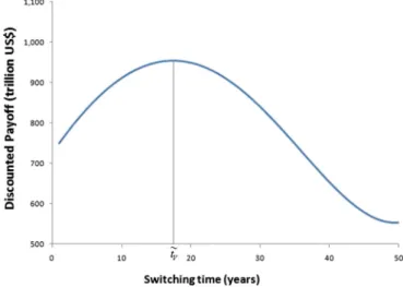
Suppose for instance that our planning horizon and discount rate werefixed at, e.g.,T= 50,r= 0.02.Fig. 1gives the payoffs of the non-forest-owner group in they-axis for each possible switching time (x-axis). We observe, for this particular case, that switching fromVmax toVminafter~tV(where~tV¼17 years) is the best course of action.

We can generalize the algorithm presented inTable 1and let the planning horizonTvary while keeping the discount raterconstant. In so doing we obtain the best switching time for each different planning horizon.

Fig. 2gives the optimal switching time for each possible planning

horizonT. To better understand thisfigure, it is important to distinguish between three elements, namely,

T:the planning horizon;

Ts:the minimum planning horizon for a switch to take place; ~

tV:the actual switching time:

The diagonal line indicates that no switch is applicable. The shortest planning horizon for which there is a switch,Ts, is thefirst element of the curve off the diagonal.Fig. 2illustrates the fact that it pays to emit more in the short run (i.e., it is optimal to increase emissionsfirst to re-duce them later and not the opposite). It also shows that for longer plan-ning horizons it is comparatively less attractive to applyVmax. This result is related to the non-linear damage functionL(S), by which the environ-mental damage increases when GHGs accumulate due to excessive emissions, on the one hand; and to the effect of increasing the damages accounted for by increasing the planning horizon, on the other.

InFig. 2,Ts_{= 38. This means that there is no switch ifTb38, and that}

there will be one ifT≥Ts_{. As mentioned before,T}s_and~t

Vdo not coincide,

even whenT=Ts_{. Put differently, if the planning horizon is long enough} the non-forest-owner group recognizes the need to switch to a cleaner regime, but the switch will take place some time before the terminal date. Note that the pairðT¼50;~tV¼17Þ, which we obtained inFig. 1,

is now just one point of the curve displayed inFig. 2.

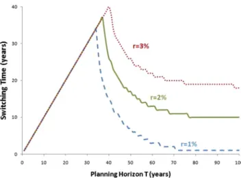
We can further generalize our algorithm for any value ofr. In the previous twofigures,rwas set equal to 0.02 (2%). The previous results are compared with two other alternative scenarios,r= 1% andr= 3%, inFig. 3.

Fig. 3conveys a dual message: First, when the discount rate is lower,

the non-owners internalize the negative externality earlier, due to the accumulation of GHGs in the atmosphere. This can be inferred from the fact thatTs_{is lower for lower discount rates. In particular, we have} thatTs= 35 ifr= 1%;Ts= 38 ifr= 2%; andTs= 41 ifr= 3%. Second, regardless of the discount rate, the longer the time horizon used, the earlier the switch, i.e., the three curves are downward sloped.

To summarize, it is optimal for the non-owners to increase emissions ifT≲40. IfT≳40, it is better to switch to a cleaner regime (V=Vmin) at some time~tV. The optimal time for the switch directly depends on the

planning horizon and the discount rate used. A simple folk conjecture says that the longer the planning horizon and/or the smaller the intertemporal discount rate, the sooner this switch will arrive. This is re-lated to the damage functionL(S), which yields greater (cumulative) losses for lower discount rates and longer planning horizons.

Table 1

Sketch of algorithm used to compute the optimal switching time~tV.

Fig. 1.Payoffs as a function of the switching time.

It is worth noting at this point that we have no prescription to make in terms of what planning horizon should be used, we simply illustrate how the optimization results change as a function of the planning hori-zon. If anything, what our results suggest is that taking into account long-term damages may lead to sensibly different optimal solutions, in this sense it seems desirable to use a longer planning horizon.

It has been shown how to determine the switching time. To put things into perspective, denote byΠthe discounted sum of instanta-neous payoffs over the planning horizon. The instantainstanta-neous payoff can be expressed in terms of the controlπ(V) and so canΠ:

ΠðV tð ÞÞ ¼ ZT

0

e−rtπðV tð ÞÞdt−ϕðS Tð ÞÞe−rT: ð18Þ

One can compare the difference in the sum of discounted payoffs for non-owners when the optimal emissions trajectory (with switch),Π ðV^Þ, is applied all along with the payoffsΠ(Vmax) andΠ(Vmin) that are obtained by applying the constant (and sub-optimal) solutions V=Vmax∀t∈[0,T] andV=Vmin∀t∈[0,T], respectively. The value

of_ΠðV^ÞinFig. 4is obtained by computing expression(18)forr= 2%

and forT∈[0, 100] along the optimal path forE(t) andS(t). Note that forTb38ΠðV^ÞandΠ(Vmax) coincide. ForT≥38 there will be a switch andΠðV^Þdiverges fromΠ(Vmax).

So far we have analyzed the optimal emissions policy. It is also im-portant to analyze the sign of the shadow price of the forest stock,λF. This shadow price is positive regardless of the time horizon and

discount rate considered. The positive sign of the co-stateλFis directly related to the ability that forests have to sequester carbon. Since the in-crease in forest area is directly related to the enhancement of carbon se-questration (see expression(9)); then, regardless of the value ofFand S,13_{marginally increasing the forest area implies marginal reductions} inE(t), meaning smaller environmental losses (see expression(11)). This is a qualitative aspect.

At the same time, we have seen that the importance of reducing emissions is directly related to the length of the planning horizon and inversely related to the discount rate. Likewise, the marginal value that non-owners attach to an additional hectare of forest is greater when the planning horizon is longer and the discount rate is lower. This is a more quantitative aspect.

In short, unlike forest owners, the non-owners are interested in in-creasing the total forest area, and this is reflected by the sign ofλF. If we compare the different ways in which forest owners and non-owners evaluate an additional hectare of forest, it is clear that there ex-ists an environmental externality. Recall that forests in our model have at least two uses: (i) the provision of economic revenues; and (ii) car-bon sequestration. These uses are competing and somewhat mutually excluding. Forest owners create a negative externality on non-owners with their net deforestation policy. Hence the question is: should this negative externality be corrected?

Given the existing property rights over the forest, and the fact that forest owners' payoffs are a decreasing function of the total forest area, reducing the net deforestation is harmful for forest owners. There-fore, the answer to this question depends on whether an additional unit of forest can generate an increase in the payoff of the non-owners, such that it more than compensates for the reduction in the forest owners' revenues when they apply a more environmentally friendly deforesta-tion/afforestation policy. If that is the case, then it will be jointly optimal to correct the externality, or at least part of it. In the next section we compute joint payoffs to answer the question raised above. We also compare the cooperative scenario to thestatus-quoindividual equilibri-um results.

4. Cooperative Solution

In the previous section we determined the non-cooperative (status-quo) strategies for both forest owners and non-owners. We saw that forest ownersfind it optimal to deforest as much as possible and to not afforest. On the other hand, non-owners suffer a negative environ-mental externality coming from the depletion of the forest via the reduced-carbon-sequestration effect. A relevant question to address is whether cooperation can improve welfare. The collectively optimal so-lution can be obtained by jointly optimizing the payoff functionals of the two players, that is,

max

0≤A tð Þ≤Amax; 0≤D tð Þ≤Dmax; Vmin≤V tð Þ≤Vmax

Z T

0

e−rt_{½R F tð ð Þ;D tð ÞÞ þG E tð ð ÞÞ−L S tðð ÞÞdt−φðS Tð ÞÞe}−rT_:

s:t:: F ð Þ ¼t A tð Þ þηF tð Þ−D tð Þ; F≥F tð Þ≥0; Fð Þ ¼0 F0;

E ð Þ ¼t V tð ÞE tð Þ; E tð Þ≥0; Eð Þ ¼0 E0;

Sð Þ ¼t E tð Þ_−ϕF tð Þ₋W_; S tð Þ_≥0_; Sð Þ ¼0 S0;

whereA,DandVare the three control variables. The joint payoff is max-imized subject to the dynamics of the forest area, emissions, and stock of greenhouse gases in the atmosphere.

Appendix E presents the optimality conditions for this cooperative problem.

As expected the optimal afforestation rate and speed of adjustment of emissions are bang-bang policies because the Lagrangian is linear in Fig. 3.Impact of the discount rate on the switching time.

Fig. 4.ComparingΠðV^ÞwithΠ(Vmin) andΠ(Vmax). 13

these variables. Further, although the co-state variable associated with the forest stock,_λFc_{, appears, as in the non-cooperative case, in the} opti-mality conditions forAandD, there is an important difference, that is,λFc now captures the negative valuation of an extra hectare of forest (forest owners) and the positive effect that increasing forest area has on carbon sequestration (non-owners). Therefore,λFc_{can take either positive or} negative values depending on which effect dominates. Furthermore, unlike in the non-cooperative case where the sign ofλFwas constant along the planning horizon for both players, now nothing prevents this sign from changing over time. Hence, it is possible that we have a switch in either the afforestation rate or the deforestation rate or in both throughout the planning horizon.

To solve forλFc_{, we need the analytical expression forF, which} de-pends on bothAandD(see (E.1)). In the non-cooperative scenario it was possible to analytically characterize the solution to the forest owners' problem by supposingex-antethat we were in the right case offigure, and then verifying,ex-post, that ourfirst-order conditions were indeed satisfied (see Appendix B for more details). This reasoning was possible because the optimal afforestation and deforestation rates were constant. In the present case however, we can have a policy switch onAand/orDat any time. Therefore, the value ofλFc

depends on the switching time onAandD. The implication is that thefirst-order condi-tions will be satisfied for allt∈[0,T]only if the exact switching time for both variables is chosen.

From (E.3) we see thatλEc_{depends onλS}c_{, and from (E.2) we have} thatSis a function ofF. Therefore, to obtainλEc_{we need to know the} evo-lution of the forest stock, which depends on the applied policies for af-forestation and deaf-forestation. As it turns out, not only do we have a potential switch of regimes for all three controls, but the switches them-selves are interdependent.

One can obtain the analytical expressions for the evolution of the state and co-state variables for all possible cases (i.e., before and after the switch). But just as it happened with the problem of the non-forest-owner group, it is not possible to derive the exact switching times analytically.

Denote now bytAc,tDcandtVcthe switching time forA,DandV, respec-tively. We evaluated the discounted intertemporal sum of joint payoffs for all possible combinations of integer switching times (tAc,tDc,tVc) using a similar algorithm as before. SeeTable 2for a sketch of the algorithm. The only difference from the previous algorithm is that now the computational complexity is increased as a consequence of the multi-plicity of cases. Denote by~tcA;~t

c D;~t

c

Vthe three integer switching times

that yield greater intertemporal payoffs. We computed~tcA;~t c D;~t

c V for

T∈{1, 2,…, 100} and forr∈{0.01, 0.02, 0.03}. Again, the results are

linked to the length of the planning horizon and the discount rate used. We observe that the solutions obtained can be classified into four different groups that coincide with four regions of the parameter space. We denote them byZ1toZ4. The boundaries of regionsZ1–Z4 are related to parameterT. We denote the limits to these regions by T1,T2andT3.

The results, which are summarized inTable 3, call for the following comments:

(i) If the problem's planning horizon is short (i.e.,TbT1) we are in regionZ1and the cooperative solution coincides with the non-cooperative one (i.e., the non-cooperative solution brings no gain). The label not applicable (N.A.) is used here to denote that there is no switching time and that the solution coincides with the sta-tus quo.

(ii) If we are in regionZ2(i.e.,T1≤TbT2), then it is jointly optimal to afforest at the maximum rate for some time and then to switch to afforestationAminat some time before the end of the planning horizon. It is not optimal to afforest all the time and we have thatAc_=Amaxiftb~_tc

AandAc=Aminift≥~t c A.

We use the notation~tc_A¼fðTÞto denote the fact that the switching time depends onT. In factf(T) is an increasing func-tion ofT. Clearly, for larger values ofT, it is optimal to switch later. The same reasoning applies for~tc_D. In this case, though, we haveD∗=Dminiftb~t

c

DandD∗=Dmaxift≥~t c D.

(iii) If we are in regionZ3(i.e.,T2≤TbT3), then it is optimal to applyA∗=AmaxandD∗=Dminall along. We have used the no-tation~tcA¼~tD¼Tto differentiate it from labelN.A.Recall that

labelN.A.was used to denote that there is no switch and that the optimal policy is identical to thestatus quoone (i.e.,Ac₌ AminandDc_=D

max∀t∈0,T]) whereas in regionZ3we also have that there is no switch, but the optimal policy is to applyAc_=AmaxandDc_{=Dminthroughout.}

(iv) Finally, regionZ4is identical to regionZ3except for the emis-sions policy. IfT≥T3then it is certain that we will have a jump fromVmaxtoVminat some point in time~tcV. The time of

the switch is also a function ofT.

The impact of cooperation is more intense and the solution is more environmentally friendly as we move from regionZ1(no gain from cooperation) to regionZ4. When the discount rate is smaller, the envi-ronmental damage is further internalized.Table 4shows the values of T1toT3for different values in the discount rates. It is not surprising that when the discount rates are smaller, the threshold planning hori-zons (T1,T2,T3) between regionsZ1,Z2,Z3andZ4are shifted downwards

(seeTable 4).14

Appendix F shows that these results seem quite robust to changes in the environmental damage parameter (parameterc).

Table 2

Sketch of the algorithm used to obtain~tcA,~t c D,~t

c V.

Table 3

Jointly optimal policies are a function ofT.

Switch Z1 Z2 Z3 Z4

~tA N.A. ~tA¼fðTÞ T T

~tD N.A. ~tD¼gðTÞ T T

~tV N.A. N.A. N.A. ~tV¼hðTÞ

14

5. Sharing the Gain of Cooperation

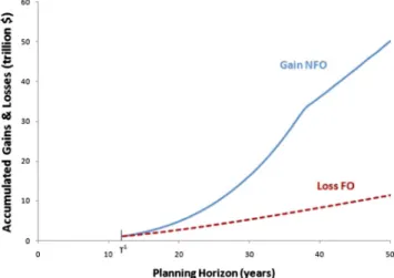
In this section, we determine a time-consistent allocation of the dividend of cooperation among the two players. We have shown that joint payoffs are greater in the cooperative setting provided thatT≥T1. This is due to the damage reduction generated by in-creased afforestation effort and lower deforestation rates. Coopera-tion, however, does not bring gains to both players. The non-forest-owner group gains from the lower environmental damage, while for-est owners lose by applying forfor-est policies that are environmentally friendly but revenue harming.

Let (xτ,τ) be the position of the game at timeτ∈[0,T] and the state-vector valuexτ. Denoted byJic(x0,t0) the payoff-to-go that play-eri∈fO;⊖gobtains if the game is played cooperatively throughout the planning horizon, and byJinc(x0,t0) its non-cooperative counter-part. The differenceJ⊖c(x0,t0)−J⊖nc(x0,t0) measures the individual

gain that non-owners obtain from cooperation. By the same tokenJnc O ðx0;t0Þ−JcOðx0;t0Þrepresents the loss that forest owners have in the

cooperative settingvis-à-visthe non-cooperative one. These two quantities are a function ofTandr. We compare the cooperative gains of non-owners and the cooperative losses of forest owners in

Fig. 5forr= 2%.

The cooperative gain by the non-forest-owner group is represented by the solid line, and the loss by forest owners by the dashed one. The vertical difference between these two lines measures the dividend of cooperation given by

DC¼ Jc

⊖ðx0;t0Þ þJcOðx0;t0Þ

− Jnc

⊖ðx0;t0Þ þJncOðx0;t0Þ

;

for any given planning horizonT. We obtain empirically thatDCN0 for T≥T1(withT1= 11 years), andDC= 0, otherwise. This means that, un-less the planning horizon is longer thanT1(which is 11 years forr= 2%), cooperation is useless. For intermediate values of T, i.e.,T1≤TbT3, we haveDCN0, and it is optimal to mitigate future dam-ages by increasing afforestation and decreasing deforestation, but not to abate emissions. If the planning horizon is sufficiently long, that is, T≥T3, then it is optimal both to mitigate (from the beginning) and to abate emissions (from time~tc_Vonwards). As emissions abatement has a greater cost than increasing afforestation or decreasing deforestation, it is preferable to start by applying less costly measuresfirst and then move into more costly ones as environmental damages increase.

Although the total dividend of cooperation is by virtue of joint opti-mization always non-negative, this does not mean that cooperation is Pareto improving. In our case, it is clear that for cooperation to be imple-mented, the non-owners need to compensate forest owners for their losses. There are many solution concepts15_{in cooperative games that} address the problem of sharingDC. We adopt here the often used Nash-bargaining procedure, which gives a unique, fair and Pareto-improving solution.16_{The Nash-bargaining solution (NBS) allocates to}

each player his non-cooperative outcome plus half of the dividend of co-operation, that is,

JNBSi ðx0;t0Þ ¼Jnci ðx0;t0Þ þ

1 2

X

i∈fO;⊖g

Jciðx0;t0Þ−Jnci ðx0;t0Þ

: ð19Þ

5.1. Time-consistent Sharing Schedule

Although the Nash-bargaining outcomes defined in Eq.(19)are Pareto-improving with respect to non-cooperative outcomes, it does not guarantee that the players will indeed continue to implement over time their part of the cooperative solution. In fact, the agreement will not be sustained if it is optimal, for at least one of them, to deviate to a non-cooperative mode of play at an intermediate dateτ∈(0,T]. This would mean that the agreement designed at the initial date for the whole duration of the game is not time consistent. (For a tutorial on time consistency in differential games, the reader may consultYeung

and Petrosjan (2005)orZaccour (2008).) Formally, we say that a

coop-erative solution (here NBS) is time consistent at (x0,t0) if, at any position (xτ∗,τ), and for allτ∈[t0,T], it holds that

JNBS

i xτ;τ≥Jnci xτ;τ; i∈fO;⊖g; ð20Þ

wherex∗denotes the cooperative state trajectory. Note that the compar-ison of payoffs-to-go in Eq.(20)at anyτ∈[t0,T] is carried out along the cooperative state trajectory, that is, under the assumption that the players have cooperated untilτ.

Solving the time-consistency problem amounts tofinding payment functionsωiðtÞ;i∈fO;⊖g;t∈½t0;T, such that the following two

proper-ties hold:

Full allocation:ZT

t0 e−rt_ω

ið Þtdt¼JNBSi ðx0;t0Þ; ð21Þ

Time consistency:JNBSi ðx0;t0Þ ¼

Z τ

t0 e−rt_ω

ið Þt dtþe−rτJiNBSxτ;τ: ð22Þ

Thefirst property states that the total payments that each player re-ceives overtime must correspond to what he is entitled to, as deter-mined by the Nash-bargaining solution. To interpret the second condition, assume that the players wish to renegotiate the initial agree-ment at (any) intermediate instant of timeτ. At this moment, the posi-tion of the game is (xτ∗,τ), meaning that cooperation has prevailed from the initial time untilτ, and that each playeriwould have been allocated a stream of monetary amounts given by thefirst right-hand-side term. Now, if the subgame starting with initial conditionx(τ) =xτ∗, is played

Fig. 5.Cooperation gains and losses by NFO and FO.

15_{For example, theKalai and Smorodinsky (1975)bargaining solution or theKalai} (1977)egalitarian principle.

16

The unfamiliar reader with the Nash-bargaining solution can consult, e.g., Wikipedia (http://en.wikipedia.org/wiki/Bargaining_problem) for a quick introduction.

Table 4

Threshold times are a function of the discount rate.

Discount T1 T2 T3

r= 1% 11 19 36

r= 2% 12 20 38

cooperatively, then playeriwill get his NBS-value component in this game given by the second right-hand-side term of Eq.(22). If what he has been allocated until_τand what he will be allocated from this date onward add up to his payoff in the original agreement, i.e., his NBS valueJiNBS(x0,t0), then a renegotiation would leave the original agree-ment unaltered. If one can_find a vector _ωðtÞ ¼ ðωOðtÞ;ω⊖ðtÞÞ such that Eq.(22)holds true, then the allocation over timeω(t) is time con-sistent. To obtain the valueωi(t),t∈[t0,T], it suffices to differentiate

Eq.(22), that is,

ωið Þ ¼τ r JNBSi xτ;τ−_dd_τ JNBSi xτ;τ

: ð23Þ

The above formula has a nice interpretation. It allocates to playeri at timeτthe interests on cooperative payoff-to-go, minus the variation over time of this payoff-to-go. We have computed forest owners' NBS payoffs-to-goðJNBSO ðxτ;τÞÞand their non-cooperative payoffs-to-goðJnc_Oðx_τ;τÞÞ. The results are plotted inFig. 6.

InFig. 6we see that the NBS outcomes (solid line) dominate their

non-cooperative deviation counterparts (dotted line) for any timeτ. This means that cooperation is time consistent and non-forest owners have no incentive to deviate from the agreement. The vertical difference between these two curves illustrates, at each point in time, the amount of money that forest owners gain by cooperating (i.e., their net cooper-ation gain-to-go). In particular, fort= 0 we obtain the net discounted gain at the beginning of the planning horizon.Fig. 6also displays forest owners' sum of discounted cooperative payoffs-to-go before transfers are applied (dashed line),Jc_Oðx_τ;τÞ. The vertical difference betweenJNBS_O

ðx_τ;τÞandJc

Oðxτ;τÞgives the value of the compensation payments-to-go. Recall that, by cooperating, forest owners reduce their deforestation and therefore suffer economic losses. The amount of money with which they are compensated has to more than cover this loss. For a more straightforward visualization of the intertemporal decomposition of these NBS compensation payments we presentFig. 7.

Fig. 7shows the yearly decomposition of the economic transfers.

These transfers, which have been discounted, are decreasing in time. The main reason why less money is required to bind forest owners into the agreement as time goes by is simply that the gain that forest owners can make by deviating from it is decreasing in time. Therefore, a lower amount is necessary. The economic interpretation is that the compensating mechanism based on the Nash-bargaining solution is time consistent, that is, cooperation is implementable and sustainable overtime.

6. Conclusions

In this paper we propose a model with two types of players: forest owners and the non-forest-owner group, where thefirst group is inter-ested in maximizing economic revenues and the second group is con-cerned with the conservation of the forest. A number of papers in the dynamic game literature (e.g.van Soest and Lensink (2000),Fredj

et al. (2004, 2006),Martín-Herrán and Tidball (2005)and

Martín-Herrán et al. (2006)) have looked at the conditions necessary to build environmental agreements that are both credible and sustainable when it comes to stopping deforestation. In these papers the environ-mentally aware players (non-forest-owners) are willing to compensate forest owners in order to have deforestation reduced.

We look at the same problem from a different angle: forests play an important role in mitigating climate change through carbon sequestra-tion. Deforestation has great impact not just in forest depletion but also on the evolution of the atmospheric stock of greenhouse gases.

There exist a number of papers in the dynamic-game literature that consider environmental damages from emissions in a dynamic setting: for example, the early papers byvan der Ploeg and de Zeeuw (1992),

Long (1992),Dockner and Long (1993), and the literature review by

Jørgensen et al. (2010), and recently,Masoudi and Zaccour (2013). In

this literature, emissions are a control variable and the issue is to deter-mine the optimal emissions rate so as to reduce the environmental damage coming from the excessive accumulation of GHGs. Typically, these models concentrate on the difficulty of coordinating optimal emission levels and treat carbon sequestration as exogenously given. We model the two issues together and account explicitly for the role of forests as a carbon sink and treat carbon sequestration not as exoge-nously given, but rather as the consequence of endogenous decisions, much in the same way as inAndrés-Domenech et al. (2011)except that here we are not in a pure control setting but there exists interaction among the players themselves.

In our proposal, forest owners have an incentive to deforest to in-crease their economic revenues, while non-owners suffer a negative ex-ternality from deforestation due to the so-called reduced-carbon-sequestration effect, which states that a tree that is cut cannot grow and hence cannot sequester carbon. We model the economic incentives of both types of players and explore the conditions that make environ-mental cooperation strictly welfare improving. Cooperation brings greener outcomes and makes it possible to partly internalize the posi-tive externality created by carbon sequestration by forests.

Three different mechanisms to reduce GHG accumulation are proposed: abatement of emissions, increases in afforestation, and de-creases in deforestation. The results show that when the perceived Fig. 6.Time consistency: non-forest-owner group.

environmental damage is small (i.e., short planning horizons and/or high intertemporal discount rates), cooperation brings little or no gain. However, as the environmental damages increase, it becomes jointly optimal to have some afforestation effort and deforestation re-duction. If the environmental damages coming from the excessive accu-mulation of greenhouse gases are suf_ficiently high, then it will be optimal to combine forestation efforts (reduced deforestation and in-creased afforestation) with emissions abatement. Reducing emissions is more expensive but also more effective in mitigating future environ-mental damage coming from the excessive accumulation of GHGs.

Our results convey a doubly positive message:first, considering for-ests' carbon-sequestration potential can make a significant difference toward stopping the destruction of the forests. Second, international co-operation can bring sound economic and environmental gains. Cooper-ation however will not arise spontaneously. For cooperCooper-ation to exist, some sort of intertemporal compensating transfer mechanism is need-ed. It is important to design this transfer mechanism correctly; other-wise the agents may have an economic incentive to withdraw from it, which in turn, will lead to worse environmental outcomes. In order for an environmental agreement to be credible, time consistency is re-quired, i.e., it has to be economically optimal for all the players involved to comply with the agreement at all times. We show that applying an intertemporal decomposition of the Nash bargaining scheme allows us to obtain time consistent outcomes.

The results obtained are very promising and can be applied to de-sign time-consistent intertemporal payments in REDD and REDD + agreements. For instance, the dichotomy used here (owners and non-owners) can be easily extended to consider countries (e.g., developing countries with forests on the one hand, and devel-oped countries willing to pay for forest conservation on the other). Also, we have modeled here the payment of one ecosystem service (carbon), the framework and methodology used lend themselves to modeling the payment for other ecosystem services such as water provision, biodiversity, land protection, etc. Since forest conserva-tion is complementary with the provision of most of these services, by including more services in our model, the range of parameters (time horizon and discount rates) for which cooperation through re-duced deforestation is overall welfare improving will increase. This in turn will imply that both the economic benefits arising from coop-eration and the amount of money to be shared will increase the greater the amount of services considered.

The conclusions arising from our work suggest that compensation schemes based on services of the same type should not be constant, but rather a decreasing function of time with greater compensation pay-ments allocated in the short run. This is the only way in which paypay-ments can credibly bind forest owners to cooperate. Some aspects such as the degree of economic development of (forestry) countries have not been explicitly modeled here. Including such aspects could only reinforce the strength of our conclusions (i.e., that transfers have to be greater in the short run, and then decrease as time goes by) since the opportunity cost to reduce deforestation is greater in a developing country where the av-erage revenue is low; see e.g., Angelsen and Rudel (2013) and Wolfersberger et al (2014).

All that being said, there are many aspects that were not considered and that call for a critical interpretation of the results: carbon sequestra-tion by the oceans may be affected by the excessive acidification of sea-water which has not been specifically modeled here. Also a more comprehensive dynamics of the accumulation of greenhouse gases should consider emissions related to land-use change. More thorough research should integrate these aspects, with yet more pessimistic con-clusions expected.

Acknowledgments

We thank three anonymous reviewers and the Editor for their helpful comments. The second author's research is partially

supported by MEC under projects ECO2011-24352 and ECO2014-52343-P co-financed by FEDER funds and the COST Action IS1104

“The EU in the new economic complex geography: models, tools and policy evaluation”. The third author's research is supported by NSERC, Canada.

Appendix A. Supplementary Data

Supplementary data to this article can be found online athttp://dx. doi.org/10.1016/j.ecolecon.2015.06.016.

References

Andrés-Domenech, P., Saint-Pierre, P., Zaccour, G., 2011.Forest conservation and CO2 emissions: a viable approach. Environ. Model. Assess. 16 (6), 519–539.

Angelsen, A., Rudel, T.K., 2013.Designing and implementing effective REDD+ policies: a 575 forest transition approach. Rev. Environ. Econ. Policy 7 (1), 91–113.

Bahn, O., Haurie, A., Malhamé, R., 2008.A stochastic control model for optimal timing of climate policies. Automatica 44, 1545–1558.

Barbier, E.B., Burgess, J.C., 2001.The economics of tropical deforestation. J. Econ. Surv. 15 (3), 413–433.

Barbier, E.B., Rauscher, M., 1994.Trade, tropical deforestation and policy intervention. En-viron. Resour. Econ. 4 (1), 75–90.

Benchekroun, H., Long, N.V., 2002.On the multiplicity of efficiency-inducing tax rules. Econ. Lett. 76, 331–336.

Breton, M., Zaccour, G., Zahaf, M., 2005.A differential game of joint implementation of en-vironmental projects. Automatica 41, 1737–1749.

Breton, M., Martín-Herrán, G., Zaccour, G., 2006.Equilibrium investment strategies in for-eign environmental projects. J. Optim. Theory Appl. 130 (1), 23–40.

Dockner, E.J., Long, N.V., 1993.International pollution control: cooperative versus nonco-operative strategies. J. Environ. Econ. Manag. 24, 13–29.

Food and Agriculture Organization of the United Nations (FAO), 2006.Global Forest Re-sources Assessment 2005.

Food and Agriculture Organization of the United Nations (FAO), 2010.Global Forest Re-sources Assessment 2010.

Fredj, K., Martín-Herrán, G., Zaccour, G., 2004.Slowing deforestation rate through subsi-dies: a differential game. Automatica 40 (2), 301–309.

Fredj, K., Martín-Herrán, G., Zaccour, G., 2006.Incentive mechanisms to enforce sustain-able forest exploitation. Environ. Model. Assess. 11 (2), 145–156.

Intergovernmental Panel on Climate Change (IPCC), 2000.Land use, land-use change and forestry. Special Report. Cambridge University Press, Cambridge.

Intergovernmental Panel on Climate Change (IPCC), 2007.Climate Change 2007: Impacts, Adaptation and Vulnerability, Fourth Assessment Report. Cambridge University Press, Cambridge.

Jørgensen, S., Martín-Herrán, G., Zaccour, G., 2010.Dynamic games in the economics and management of pollution. Environ. Model. Assess. 15 (6), 433–467.

Kalai, E., 1977.Proportional solutions to bargaining situations: intertemporal utility com-parisons. Econometrica 45 (7), 1623–1630.

Kalai, E., Smorodinsky, M., 1975.Other solutions to Nash's bargaining problem. Econometrica 43 (3), 513–518.

Le Quéré, C., Raupach, M.R., Canadell, J.G., Marland, G., et al., 2009.Trends in the sources and sinks of carbon dioxide. Nat. Geosci. 2, 831–836.

Long, N.V., 1992.Pollution control: a differential game approach. Ann. Oper. Res. 37, 283–296.

Martín-Herrán, G., Tidball, M., 2005.Transfer mechanisms inducing a sustainable forest exploitation. In: Deissenberg, C., Hartl, R. (Eds.), Optimal Control and Dy-namic Games: Applications in FinanceManagement Science and Economics. Springer, The Netherlands, pp. 85–103.

Martín-Herrán, G., Cartigny, P., Motte, E., Tidball, M., 2006.Deforestation and foreign transfers: a Stackelberg differential game approach. Comput. Oper. Res. 33 (2), 386–400.

Masoudi, N., Zaccour, G., 2013.A differential game of international pollution control with evolving environmental costs. Environ. Dev. Econ. 18, 680–700.

Van der Ploeg, F., De Zeeuw, A., 1992.International aspects of pollution control. Environ. Resour. Econ. 2 (2), 117–139.

Van Soest, D., Lensink, R., 2000.Foreign transfers and tropical deforestation: what terms of conditionality? Am. J. Agric. Econ. 82 (2), 389–399.

Wolfersberger, J., Amacher, G.S., Delacote, P., Dragicevic, A., 2014.Dynamics of deforesta-tion and reforestadeforesta-tion in a developing economy. Working Paper Chaire Economie du Climat.

Yeung, D.W.K., Petrosjan, L.A., 2005.Cooperative Stochastic Differential Games. Springer, New York.