Avoiding order reduction when integrating linear
initial boundary value problems with Lawson
methods
I. Alonso-Mallo
∗, B. Cano
†IMUVA, Departamento de Matem´atica Aplicada,
Facultad de Ciencias, Universidad de Valladolid,
Paseo de Bel´en 7, 47011 Valladolid,
Spain
and
N. Reguera
‡IMUVA, Departamento de Matem´aticas y Computaci´on,
Escuela Polit´ecnica Superior, Universidad de Burgos,
Avda. Cantabria, 09006 Burgos,
Spain
Abstract
Exponential Lawson methods are well known to have a severe order reduction when integrating stiff problems. In a previous paper, the precise order observed with Lawson methods when integrating linear problems is justified in terms of different conditions of annihilation on the boundary. In fact, the analysis of con-vergence with all exponential methods when applied to parabolic problems has always been performed under assumptions of vanishing boundary conditions for the solution. In this paper, we offer a generalization of Lawson methods in order to approximate problems with nonvanishing and even time-dependent boundary values. This technique is cheap and allows to avoid completely order reduction independently of having vanishing or non-vanishing boundary conditions.
1
Introduction
The advantages of using exponential methods when integrating in time partial differ-ential equations are clear from the literature [11, 12, 14]. As they integrate the linear
∗Email: [email protected]
and stiff part of the differential equation in an exact way, methods which are explicit and linearly stable at the same time are achieved when integrating such type of prob-lems, which is not possible with classical methods. However, up to our knowledge, exponential methods have always been applied and analysed to integrate partial dif-ferential problems under the assumption of vanishing or periodic boundary conditions. Nonvanishing boundary conditions have not been considered.
Moreover, one of the oldest particular types of exponential methods (Lawson meth-ods [12]), which are very easy to construct from a Runge-Kutta method, have many times been excluded from the analysis [10]. (They do not even satisfy the condition of stiff order 1 for the methods considered in that paper.) In any case, a recent manuscript of the authors [4] makes a thorough study of the precise order which these methods show when integrating linear problems, which strongly depends on several conditions of annihilation on the boundary of its solution.
On the other hand, for classical methods which do have stages, such as Runge-Kutta, Fractional-Step-Runge-Runge-Kutta, Runge-Kutta-Nystr¨om or Rosenbrock methods, some techniques have been suggested in the literature to avoid order reduction [2, 3] when integrating linear problems. These techniques are based on applying the method of lines by integrating first in time and then in space. Then, for the elliptic prob-lems which the stages define, appropiate boundary conditions must be considered. It happens that, in the exponential case, when the problem is linear, the stages are not relevant since they are not necessary for the calculation of the numerical solution at each step. Therefore, another strategy is necessary.
In this paper, in the first place, we give a technique to deal with the problem of nonvanishing boundary conditions when integrating linear problems with Lawson methods. Moreover, we assume that the differential operator is the infinitesimal gen-erator of a C0-semigroup and, in this way, both hyperbolic and parabolic cases are included. Secondly, we prove that the suggested technique allows to avoid order reduc-tion completely. More precisely, the order observed is that of the underlying classical Runge-Kutta method when applied to a non-stiff problem. Besides, this technique is not expensive as it just implies to add some terms concerning boundary values which are negligible in number compared to the values to approximate in the interior of the domain. In such a way, it is not necessary to resort to methods of high stiff order (and necessarily more stages) if high accuracy is required. We also want to remark here that it is not an aim of this paper to study how to calculate in the most efficient way the necessary terms to avoid order reduction. That could be a subject of future research.
discretizations.
2
Preliminaries
Let X and Y be two complex Banach spaces, D(A) a dense subspace of X and A :
D(A)⊆X →X,∂ :D(A)⊆X →Y a pair of linear operators. We consider the linear abstract initial boundary value problem
u′(t) = Au(t) +f(t), u(0) = u0,
∂u(t) = g(t),
(1)
whereA and ∂ satisfy the following assumptions:
(A1) The boundary operator ∂ :D(A)⊂X →Y is onto.
(A2) Ker(∂) is dense inX and A0 :D(A0) = ker(∂)⊂X →X, the restriction of A to Ker(∂), is the infinitesimal generator of a C0- semigroup {etA0}
t≥0 in X, which type is denoted by ω.
(A3) If z ∈C satisfiesRe(z)> ω and v ∈Y, then the steady state problem
Ax = zx,
∂x = v, (2)
possesses a unique solution denoted by x=K(z)v. Moreover, the linear operator
K(z) :Y →D(A) satisfies
∥K(z)v∥X ≤L∥v∥Y, (3)
where the constant L holds for any z such thatRe(z)> ω0 > ω.
With these assumptions, the problem (1) is well-posed in BV /L∞ sense [16]: (WP1) If u0 ∈ D(A), g : [0, T] → Y is smooth enough with ∂u0 = g(0), and f ∈
C1([0, T], X), then there exists a unique solution u∈C1([0, T], X) of (1), and
(WP2) there exist constants M >0 and α= max(ω,0) such that, for 0≤t ≤T,
∥u(t)∥X ≤M eαt
(
∥u0∥X +∥g(0)∥Y +
∫ T
0
∥g′(s)∥Yds+
∫ T
0
∥f(s)∥Xds
) .
Remark 1. Instead of (A3), we can impose equivalently,
(A3’) The operator (A, ∂) :D(A)⊂X →X×Y is closed.
Remark 2. Although the previous well-posedness is sufficient for our analysis, it is
possible to prove the well-posedness of the problem (1) when other norms ofLp-type are
Remark 3. From now on, we assume for the sake of simplicity that the type ω of the semigroup{etA0}
t≥0 is negative. As a consequence, the semigroup decays exponentially
when t → 0. Moreover, the operator A0 is invertible and, since we can take z = 0 in
(2), the operator K(0) :Y →D(A)⊂X is well defined and it is continuous.
Because of hypothesis (A2), {φj(tA0)}∞j=0 are bounded operators for t >0, where
{φj} are the standard functions used in exponential methods [11], which are defined
by
φj(tA0) = 1
tj
∫ t
0
e(t−τ)A0 τ j−1
(j−1)!dτ, (4)
and can be calculated in a recursive way through the formula
φk+1(z) =
φk(z)−1/k!
z , z ̸= 0, φk+1(0) =
1
(k+ 1)!, φ0(z) =e
z
. (5)
These functions are well known to be bounded on the complex plane when Re(z)≤0. Since we are interested in approximations of high order, we assume that the solution of (1) is regular. We will assume that, for a natural number p,
Ap+1−ju(j) ∈C([0, T], X), 0≤j ≤p+ 1. (6) This assumption implies that the time derivatives of the solution are regular in space, but without to impose any restriction on the boundary values. Theorem 3.1 in [1] shows that this is satisfied when the data u0, f and g are regular and the boundary values ∂u0, ∂f(0) and g(0) satisfy certain natural compatibility constraints. As a consequence, from (1),
u(j)(t) =
j−1
∑
l=0
Alf(j−1−l)(t) +Aju(t), 0≤j ≤p+ 1, (7)
which implies that the boundary values
∂Aju(t) =g(j)(t)−
j−1
∑
l=0
∂Alf(j−1−l)(t), 0≤j ≤p+ 1, (8)
can be obtained from the data of the problem (1). These boundary values are crucial in our analysis below.
For the time integration, we will center on Lawson methods [12], which applied to a finite-dimensional linear problem like
U′(t) = BU(t) +F(t), (9) whereB is a matrix, are described by the following formula at each step
Un+1 =ekBUn+k s
∑
i=1
Here, the coefficients {bi},{ci} are those of an underlying Runge-Kutta method. For
this problem, they just correspond in fact to a quadrature rule approximation to the integral in the equality
U(tn+1) = ekBU(tn) +k
∫ 1
0
ek(1−s)BF(tn+sk)ds, (11)
which is satisfied by the solutions of (9) when tn+1 = tn+k. Notice that, when the
method has order p, the corresponding quadrature rule exactly integrates all polyno-mials of degree ≤ p−1. (As distinct, notice that, with exponential quadrature rules,
F is approximated by a polynomial and then the integral is performed exactly.)
3
Time semidiscretization
In this section, we give the technique to avoid in time order reduction with vanishing and non-vanishing boundary conditions. Besides, we prove the full-order convergence for the local error of the time semidiscretization.
3.1
Description of the technique
Our idea is to generalize the exponential Lawson method (10) to be able to use it to time integrate the initial boundary value problem (1).
When the boundary values vanish, in which case A ≡ A0 is the infinitesimal gen-erator of a C0-semigroup, the method (10) can be generalized in an obvious way by taking etA0 as the semigroup generated by A0.
The key in order to include non vanishing boundary values is to realize thatv(t) =
etA0α is the solution of the abstract differential problem
v′(t) = A0v(t),
v(0) = α,
which, with the notation of (1), corresponds to the initial boundary value problem
v′(t) = Av(t), v(0) = α ∂v(t) = 0.
(12)
Then, we add suitable boundary values to (12) and we replace v(t) =etA0α in the
exponential Lawson method with its solution. If we choose the boundary values
v′(t) = Av(t), v(0) = α,
∂v(t) = ∑pj=0 tjj!∂Ajα,
we deduce that
v(k) =
p
∑
j=0
kj
j!A
(see Lemma 4) and we can prove the consistency of orderp for the whole method just as in the case of an ordinary differential system (see Theorem 7.)
With this idea, for the time integration of (1) we suggest to advance a stepsize from
un in the following way
un+1 = ˆun,0 +k
s
∑
i=1
bifˆn,i, (13)
where ˆun,0 is the value at t=k of the solution of
u′n,0(t) = Aun,0(t),
un,0(0) = un,
∂un,0(t) =
∑p
j=0
tj j!∂A
ju(t n),
(14)
and ˆfn,i is the value at t =k(1−ci) of the solution of
fn,i′ (t) = Afn,i(t),
fn,i(0) = f(tn+cik),
∂fn,i(t) =
∑p−1
l=0
tl l!∂A
lf(t
n+cik).
(15)
We notice that the boundary values in (14) can always be calculated in terms of data taking (8) into account.
3.2
Local error of the time semidiscretization
In order to study the local error, we consider the value obtained in (13) starting from
u(tn) in (14), and (15). Then, we obtain
un+1 = ˆun,0 +k
s
∑
i=1
bifˆn,i,
where ˆun,0 is the value at t=k of the solution of
u′n,0(t) = Aun,0(t),
un,0(0) = u(tn),
∂un,0(t) = ∂(
∑p
j=0
tj j!A
ju(t n)),
(16)
and ˆfn,i is that defined in (15).
To bound the local errorρn+1 = ¯un+1−u(tn+1), we use the following lemma
Lemma 4. Let us assume hypotheses (A1)-(A2)-(A3) of Section 2, and thatα∈D(A),
β∈D(Ap+1) satisfy ∂α=∂β. Consider the auxiliary problem
v′(t) = Av(t), v(0) = α, ∂v(t) = ∂z(t),
where
z(t) =
p
∑
j=0
tj
j!A
jβ.
Then,
v(t) =etA0(α−β) + p
∑
j=0
tj
j!A
jβ+tp+1φ
p+1(tA0)Ap+1β (18)
and
Av(t) =etA0A
0(α−β) +
p−1
∑
j=0
tj
j!A
j+1β+tpφ
p(tA0)Ap+1β,
where φp(z) and φp+1(z) are defined in (4).
Proof. By considering w(t) =v(t)−z(t) one gets
w′(t) =A0w(t) +
tp p!A
p+1β, w(0) =α−β,
which means that
w(t) = etA0(α−β) +
∫ t
0
e(t−τ)A0τ p
p!A
p+1βdτ,
and (18) follows. Now, we can apply Lemma 1 in [4] (see also [17]) and we deduce that
∫ t
0
e(t−τ)A0τ p
p!A
p+1βdτ ∈D(A 0)
and
A0
∫ t
0
e(t−τ)A0τ p
p!A
p+1βdτ = −t
p
p!A
p+1β+
∫ t
0
e(t−τ)A0 τ p−1 (p−1)!A
p+1βdτ,
which proves the second formula.
From this result, we can study more thoroughly ¯un,0(t) and fn,i(t).
Lemma 5. Let us assume hypotheses (A1)-(A2)-(A3)-(WP1)-(WP2) of Section 2.
Then,
un,0(t) =
p
∑
j=0
tj
j!A
ju(t
n) +tp+1φp+1(tA0)Ap+1u(tn),
and
Aun,0(t) =
p−1
∑
j=0
tj
j!A
j+1u(t
Lemma 6. Let us assume hypotheses (A1)-(A2)-(A3)-(WP1)-(WP2) of Section 2. Then,
fn,i(t) = p−1
∑
j=0
tj j!A
j
f(tn+cik) +tpφp(tA0)Apf(tn+cik).
and
Afn,i(t) = p−2
∑
j=0
tj
j!A
j+1f(t
n+cik) +tp−1φp−1(tA0)Apf(tn+cik).
We now deduce the consistency of order p.
Theorem 7. Under hypotheses (A1)-(A2)-(A3)-(WP1)-(WP2) of Section 2, and
as-suming that u(t) ∈ D(Ap+1) for t ∈ [0, T], with Aju ∈ C([0, T], X), j = 0, . . . , p+ 1, and f(l)(t) ∈ D(Aj) for t ∈ [0, T], with Ajf(l)(t) ∈ C([0, T], X), l = 0, . . . , p+ 1−j,
j = 1, . . . , p, whenever the method has order p, the local error satisfies
ρn+1 ≡un+1−u(tn+1) = O(kp+1).
where the constant in Landau notation for the residue depends on a bound for Ap+1u,
Apf, Ajf(p−j), j = 0, . . . , p−1, and the bound for the operatorsφp+1(kA0) andφp((1−
ci)kA0).
Proof. By considering t=k in Lemma 5 andt = (1−ci)k in Lemma 6, it is clear that
¯
un+1 =
p
∑
j=0
kj j!A
ju(t n) +k
s
∑
i=1
bi p−1
∑
j=0
kj(1−ci)j
j! A
jf(t
n+cik) +O(kp+1).
where the residue depends on Ap+1u, Apf and the bound for the operatorsφp+1(kA0)
and φp((1−ci)kA0). This can be rewritten as
¯
un+1 = u(tn) + p ∑ j=1 kj j! [
Aju(tn) +j s
∑
i=1
bi(1−ci)j−1 p−j
∑
l=0
clikl l! A
j−1f(l)(t
n)
]
+O(kp+1)
= u(tn) + p ∑ ˜ȷ=1 k˜ȷ ˜ȷ! [
A˜ȷu(tn) +
˜ȷ−1
∑
l=0
˜ȷ(˜ȷ−1). . .(˜ȷ−l)
l! (
s
∑
i=1
bi(1−ci)˜ȷ−l−1cli)A
˜ȷ−l−1
f(l)(tn)
]
+O(kp+1), (19)
where the change of variables ˜ȷ =j+l has been used for the second term in the bracket of (19), and the residue now also depends on a bound for Ajf(p−j), j = 0, . . . , p−1. Now, it suffices to take into account that the quadrature rule which is associated to the method integrates exactly polynomials of degree≤p−1. Then, for ˜ȷ≤p,
s
∑
i=1
bi(1−ci)˜ȷ−l−1cli =
∫ 1
0
(1−x)˜ȷ−l−1xldx= l!
where integration-by-parts has been used for the second equality. This implies, from (19) and (7), that
¯
un+1 = u(tn) + p
∑
˜ȷ=1
k˜ȷ ˜ȷ!
[
A˜ȷu(tn) +
˜ȷ−1
∑
l=0
A˜ȷ−l−1f(l)(tn)
]
+O(kp+1)
= u(tn) + p
∑
˜ȷ=1
k˜ȷ ˜ȷ!u
(˜ȷ)(t
n) +O(kp+1) = u(tn+1) +O(kp+1),
which proves the theorem.
4
Full discretization
In this section, we study the full discretization of problem (1). A crucial point is to take into account that the boundary values are nonvanishing.
When problem (1) has homogeneous boundary conditions, it can be written as the initial value problem
u′(t) = A0u(t) +f(t),
u(0) = u0,
(20)
where, in our more general approach, the operatorA0 :D(A0)⊂X →X is the gener-ator of a C0-semigroup. To reduce a problem with nonvanishing boundary conditions to one of that type, we need to assume that it is possible to find a suitable extension of the boundary value data to the whole domain where the solution is defined. That is, for eacht∈[0, T], the boundary valueg(t) is extended to an element xg(t)∈D(A)
such that ∂xg(t) = g(t). Then, the function v(t) = u(t)−xg(t) satisfies the initial
boundary value problem
v′(t) = u′(t)−xg′(t) =Au(t) +f(t)−x′g(t) =Av(t) +f(t)−x′g(t) +Axg(t),
v(0) = u(0)−xg(0),
∂v(t) = ∂u(t)−∂xg(t) = 0,
which can be written as (20).
However, this is not a practical way to obtain a numerical approximation since, at least, two problems come up when this idea is carried out. Firstly, the extension operator is not easily obtained. A possibility is to consider the extension operator
xg(t) = K(0)g(t) in (3), but it is not easy at all to obtain it for multidimensional
problems. Moreover, approximating it in a numerical way at each step would lead to the necessity of solving a linear system at each step and to numerically calculate
x′g(tn). Secondly, it is necessary to choose carefully xg(t) in order to avoid completely
the order reduction phenomenon. For example, the choice xg(t) = K(0)g(t) only
As a suitable alternative, we use a spatial discretization which takes into account the boundary values in a natural way (cf. with [1, 2]).
4.1
Spatial discretization
We first consider an abstract spatial discretization. As we will check in the examples of Section 5, this framework includes problems which are discretized in space by usual Galerkin finite element and finite difference techniques.
Let us denote by h∈(0, h0] the parameter of the spatial discretization. LetXh be
a family of finite dimensional spaces, approximatingX. The norm inXh is denoted by
∥·∥h. We suppose that
Xh =Xh,0⊕Xh,b
in such a way that the internal approximation is collected in Xh,0 and Xh,b accounts
for the boundary values.
The elements in D(A0), which are regular in space and have vanishing boundary conditions, can be approximated in Xh,0. However, it is possible to consider elements
u ∈ X which are regular in space but with non-vanishing boundary conditions, i.e.
u∈D(A). Then, it is necessary to use the whole discrete space Xh.
Since the solution is known at the boundary, our goal is to obtain a value in Xh,0 which is a good approximation inside the domain.
Let us take a projection operator
Lh :X →Xh,0.
When x ∈ D(A0), Lhx will be its best approximation in Xh,0. We also assume that there exists another operator
Qh :Y →Xh,b,
which permits to discretize spatially the boundary values. Then, we define
Ph := (Lh−LhQh∂) :D(A)→Xh,0
which is the internal spatial approximation of an element inD(A).
On the other hand, the operatorA:D(A)⊂X →X is approximated by means of the operators
Ah :Xh →Xh,0,
in such a way that Ah,0 : Xh,0 → Xh,0, the restrictions of Ah to the subspaces Xh,0, are approximations ofA0 :D(A0)⊂ D(A) → X. Therefore, when xh =xh,0 +xh,b ∈
Xh,0⊕Xh,b =Xh, we have
We pose the following semidiscrete problem: Find Uh(t)∈Xh,0 such that
Uh′(t) +LhQhg′(t) = Ah(Uh(t) +Qhg(t)) +Lhf(t),
Uh(0) +LhQhg(0) = Lhu(0),
or, equivalently,
Uh′(t) = Ah,0Uh(t) +AhQhg(t) +LhQh(∂f(t)−g′(t)) +Phf(t),
Uh(0) = Phu(0),
(21)
which results from the discretization in space of problem (1).
The subsequent analysis is carried out under the following hypotheses, which are very close to those in [6] (see also [1]).
(H1) The operatorsAh,0 are invertible and generate uniformly boundedC0-semigroups
etAh,0 on X
h,0 satisfying
||etAh,0||
h ≤M, (22)
where M ≥1 is a constant.
(H2) For eachu∈X,
∥Lhu∥h ≤C∥u∥X, (23)
where C is constant, and, for each v ∈Y,
∥Qhv∥h ≤γh∥v∥Y, (24)
where γh may increase in a moderate way when h→0.
(H3) We define the elliptic projection Rh :D(A)→Xh,0 as follows. Ifu∈D(A), then
Rhu satisfies
Ah(Rhu+Qh∂u) = LhAu, (25)
or, equivalently,
Rhu=A−h,10(LhAu−AhQh∂u).
Notice that the elliptic projection Rhu is the discretized solution of the steady
state problem with exact solution u.
We assume that there exists a subspace Z of X, such that, for u∈Z,
(a) A−01u∈Z and etA0u∈Z, fort ≥0,
(b) for some εh which is small with h,
∥(Lh−LhQh∂)u−Rhu∥h =∥Phu−Rhu∥h ≤εh∥u∥Z, (26)
4.2
Time integration. Lawson methods.
We now obtain a full discretization of (1). Notice that, since (21) is in practice an ordinary differential system, it is possible to obtain a full discretization by applying a standard Lawson method to it. However, this method comes to a very inaccurate result due to the high order reduction phenomenon arising when nonvanishing boundary values are present. (Wheng ̸= 0, the source term in (21) is, in practice, infinitely large whenh goes to zero.)
Our idea is to begin with the time semidiscretization (13) by using the solutions of problems (14) and (15). Then, we apply the space discretization described above to those problems and we obtain the scheme
Uh,n+1 = ˆUh,n,0+k
s
∑
j=1
bjFˆh,n,j, (27)
where ˆUh,n,0 equals Uh,n,0(k) with Uh,n,0(t)∈Xh,0 the solution of
Uh,n,′ 0(t) +LhQh∂u′n,0(t) = Ah(Uh,n,0(t) +Qh∂un,0(t)),
Uh,n,0(0) = Uh,n,
(28)
and un,0 is the same as in (14) and, for i = 1, . . . , s, ˆFh,n,i = Fh,n,i((1 −ci)k) with
Fh,n,i(t)∈Xh,0 the solution of
Fh,n,i′ (t) +LhQh∂fn,i′ (t) = Ah(Fh,n,i(t) +Qh∂fn,i(t)),
Fh,n,i(0) +LhQh∂f(tn+cik) = Lhf(tn+cik),
(29)
where fn,i is the same as in (15). Moreover, we will assume that we take, as initial
condition,
Uh,0 =Phu(0). (30)
4.2.1 Final formula for the implementation
Theorem 8. The numerical solution in (27) can be written as
Uh,n+1 = ekAh,0Uh,n+ p
∑
j=1
kjφj(kAh,0)[AhQh∂Aj−1u(tn)−LhQh∂Aju(tn)]
+kp+1φp+1(kAh,0)AhQh∂Apu(tn)
+k s ∑ i=1 bi [
e(1−ci)kAh,0P
hf(tn+cik)
+
p−1
∑
l=1
(1−ci)lklφl((1−ci)kAh,0)[AhQh∂Al−1f(tn+cik)−LhQh∂Alf(tn+cik)]
+(1−ci)pkpφp((1−ci)kAh,0)AhQh∂Ap−1f(tn+cik)
]
, (31)
where u(tn) is the solution of (1) we want to approximate and ∂Aju(tn) is calculated
in terms of the data g and f of (1) through (8).
Proof. Integrating exactly (28) and (29), using the boundary values in (14)-(15) and the definition of the functions {φj} (4), the method can be written as
Uh,n+1 = ekAh,0Uh,n+
∫ k
0
e(k−s)Ah,0[A
hQh∂un,0(s)−LhQh∂u′n,0(s)]ds
+k s ∑ i=1 bi [
e(1−ci)kAh,0P
hf(tn+cik)
+
∫ (1−ci)k
0
e(k−s)Ah,0[A
hQh∂fn,i(s)−LhQh∂fn,i′ (s)]ds
]
= ekAh,0U h,n+
p
∑
j=0
kj+1φj+1(kAh,0)AhQh∂Aju(tn)
−
p
∑
j=1
kjφj(kAh,0)LhQh∂Aju(tn)
+k s ∑ i=1 bi [
e(1−ci)kAh,0P
hf(tn+cik)
+
p−1
∑
l=0
(1−ci)l+1kl+1φl+1((1−ci)kAh,0)AhQh∂Alf(tn+cik)
−
p−1
∑
l=1
(1−ci)lklφl((1−ci)kAh,0)LhQh∂Alf(tn+cik)
] ,
from what the result follows.
space and the following vanishing boundary conditions are satisfied
∂u(t) =∂Au(t) =...=∂Apu(t) = 0.
This is in correspondance with the fact that the standard Lawson method in such a case is like (31) but eliminating all terms which contain the functions{φj}. This comes from
the fact that, applying the space discretization to (1) in such a case and considering (21), the following problem arises
Uh′(t) =Ah,0Uh(t) +Phf(t).
Time integration with (10) explains the remark.
Remark 10. We remark that, for many space discretizations, for v ∈Y, AhQhv and
LhQhv are local in the sense that they vanish in the interior of the domainΩ (or great
part of it). In such a way, the calculation of the terms which contain the functions
{φj} is much cheaper than it could be expected at first sight. Just some columns of the
matrices which represent φj(skAh,0) are necessary. That is thoroughly explained with
an example in Subsection 5.3.1.
4.2.2 Local errors
In order to define the local error, we consider
Uh,n+1 =Uˆh,n,0+k
s
∑
j=1
bjFˆh,n,j,
whereUˆh,n,0 equals Uh,n,0(k), withUh,n,0(t) the solution of
U′h,n,0(t) +LhQh∂u′n,0(t) = Ah(Uh,n,0(t) +Qh∂un,0(t)),
Uh,n,0(0) = Rhu(tn),
(32)
and, forj = 1, . . . , s,Fˆh,n,j =Fh,n,j((1−cj)k) with Fh,n,j(t) the solution of
F′h,n,j(t) +LhQh∂fn,j′ (t) = Ah(Fh,n,j(t) +Qh∂fn,j(t)),
Fh,n,j(0) = Rhf(tn+cjk).
(33)
We now define the local error att=tn as
ρh,n =Rhu(tn)−Uh,n,
and study its behaviour in the following theorem.
Theorem 11. Under the assumptions of Section 2, if u and f in (1) satisfy
for the spaceZ which is introduced in (H3) and the method has order p,
ρh,n+1 =O(εhkp+1+kp+1+γhkp+1) +O(kεh) =O(γhkp+1+kεh),
where εh and γh and are those in (24)-(26) and the constants in Landau notation are
independent of k and h. (In fact, they do depend on bounds for Aju, j = 1, . . . , p+ 1,
Ajf, j = 1, . . . , p and φ
j(sA0), j =p−1, p, p+ 1.)
Proof. From the definition of ρh,n,
ρh,n+1 = Rhu(tn+1)−Uh,n+1
= (Rhu(tn+1)−Rhun+1) + (Rhun+1−Uh,n+1).
Notice that, using (34), Lemmas 5 and 6, hypothesis (a) in (H3), and the recursive definition of the functionsφj(z) (5), we deduce thatρn+1 ∈Z. Then, for the first term in parenthesis and using Theorem 7, (23)-(24) and (26),
Rhu(tn+1)−Rhun+1 = Rhρn+1
= (Rh−Ph)ρn+1+Lhρn+1−LhQh∂ρn+1 = O(εhkp+1+kp+1+γhkp+1),
Moreover, the implicit constant in Landau notation is independent of k and h. Now, we apply the operator Rh to (16) and use (25),
Rhu′n,0(t) +LhQh∂u′n,0(t) = RhAun,0(t) +LhQh∂u′n,0(t)
= LhAun,0(t) + (Rh−Lh)Aun,0(t) +LhQh∂Aun,0(t) = Ah(Rhun,0(t) +Qh∂un,0(t)) + (Rh−Ph)Aun,0(t)
Rhun,0(0) = Rhu(tn).
(35)
Then, subtracting (35) from (32),
U′h,n,0(t)−Rhun,′ 0(t) = Ah,0(Uh,n,0(t)−Rhun,0(t)) + (Ph−Rh)Aun,0(t),
Uh,n,0(0)−Rhun,0(0) = 0.
Solving this problem exactly,
Uh,n,0(k)−Rhun,0(k) =
∫ k
0
e(k−τ)Ah,0(P
h−Rh)Aun,0(τ)dτ,
which is O(kεh) according to (22) and (26) in hypothesis (H3). This can be applied
becauseAun,0(τ)∈Z due to (34) and Lemma 5. In a similar way,
Rhfn,j′ (t) +LhQh∂fn,j′ (t) = RhAfn,j(t) +LhQh∂fn,j′ (t)
= LhAfn,j(t) + (Rh−Lh)Afn,j(t) +LhQh∂Afn,j(t)
= Ah(Rhfn,j(t) +Qh∂fn,j(t)) + (Rh−Ph)Afn,j(t),
and, subtracting from (33),
F′h,n,j(t)−Rhfn,j′ (t) = Ah,0(Fh,n,j(t)−Rhfn,j(t)) + (Ph −Rh)Afn,j(t),
Fh,n,j(0)−Rhfn,j(0) = Rhf(tn+cjk)−Rhf(tn+cjk) = 0.
Solving this problem exactly,
Fh,n,j(k)−Rhfn,j(k) =
∫ k
0
e(k−τ)Ah,0(P
h−Rh)Afn,j(τ)dτ,
which isO(kεh) again through the same argument as above. (We take now into account
that Afn,j(τ)∈Z due to (34) and Lemma 6.)
Therefore, we deduce that
Rhun+1−Uh,n+1 =Rhuˆn,0−Uˆh,n,0+k
s
∑
j=1
bj(Rhfˆn,j −Fˆh,n,j) =O(kεh).
4.2.3 Global errors
We now study the global errors att=tn, which are given by
eh,n=Phu(tn)−Uh,n.
Theorem 12. Under the same assumptions of Theorem 11,
eh,n =O(γhkp+εh),
where γh and εh are those in (24)-(26) and the constants in Landau notation are
in-dependent of k and h.
Proof. Because of its definition, eh,n+1 can be decomposed as
eh,n+1 = Phu(tn+1)−Uh,n+1
= (Phu(tn+1)−Rhu(tn+1)) +Rhu(tn+1)−Uh,n+1 = O(εh) +Rhu(tn+1)−Uh,n+1,
where (26) has been used. Besides,
Rhu(tn+1)−Uh,n+1 = Rhu(tn+1)−Uh,n+1+Uh,n+1−Uh,n+1 = ρh,n+1+Uh,n+1−Uh,n+1.
We now study Uh,n+1−Uh,n+1. Subtracting and considering the previous subsection,
Uh,n+1−Uh,n+1=Uˆh,n,0−Uˆh,n,0+k
s
∑
j=1
Due to (32) and (28),Uˆh,n,0−Uˆh,n,0 is the value at t=k of the solution of
U′h,n,0(t)−Uh,n,′ 0(t) = Ah,0(Uh,n,0(t)−Uh,n,0(t)),
Uh,n,0(0)−Uh,n,0(0) = Rhu(tn)−Uh,n,
and, therefore, solving exactly,
ˆ
Uh,n,0 −Uˆh,n,0 =Uh,n,0(k)−Uh,n,0(k) = ekAh,0(Rhu(tn)−Uh,n).
Similarly, from (29) and (33),Fˆh,n,j−Fˆh,n,j is the value att = (1−cj)k of the solution
of
F′h,n,j(t)−Fh,n,j′ (t) = Ah,0(Fh,n,j(t)−Fh,n,j(t)),
Fh,n,j(0)−Fh,n,j(0) = (Rh−Ph)f(tn+cjk).
Solving this problem exactly,
ˆ
Fh,n,j −Fˆh,n,j =Fh,n,j((1−cj)k)−Fh,n,j((1−cj)k) =e(1−cj)kAh,0(Rh−Ph)f(tn+cjk).
Finally, we deduce from this, Theorem 11 and (26), the following recursion formula
Rhu(tn+1)−Uh,n+1
= ρh,n+1+Uh,n+1−Uh,n+1
= ρh,n+1+Uˆh,n,0−Uˆh,n,0+k
s
∑
j=1
bj(Fˆh,n,j −Fˆh,n,j)
= ρh,n+1+ekAh,0(Rhu(tn)−Uh,n) +k s
∑
j=1
bje(1−cj)kAh,0(Rh−Ph)f(tn+cjk)
= ekAh,0(R
hu(tn)−Uh,n) +O(γhkp+1) +O(kεh).
This implies that
Rhu(tn)−Uh,n=etnAh,0(Rhu(0)−Uh,0) +O(γhkp+ϵh),
which, together with (30) and (22), proves the theorem.
5
Examples and numerical results
5.1
Parabolic problem formulation
Our main reference for this section is [18]. The references [8, 9, 20, 21, 22] are also of interest.
Let Ω be a bounded domain inRd(d= 1,2,3) with a Lipschitz continuous boundary
∂Ω. We consider the second order linear operator
Aw:=
d
∑
i,j=1
Di(aijDjw)− d
∑
i=1
(Di(biw) +ciDiw)−a0w,
where Di = ∂x∂
i. We assume that the coefficients aij(x), bi(x), ci(x) and a0(x) are
real smooth functions on the domain Ω and −A is elliptic, i.e. there exists a constant
α0 >0 such that
d
∑
i,j=1
aij(x)ξiξj ≥α0|ξ|2,
for all ξ∈Rd and almost every x∈Ω.
From the operator A, we derive the bilinear form
a(w, v) :=
∫
Ω
[ d
∑
i,j=1
aij
∂w ∂xj
∂v ∂xi
−
d
∑
i=1
(biwDiv−civDiw) +a0wv
] ,
forv, w∈V, which is a suitable subspace of functions defined over Ω. In the case of a Dirichlet problem, we take V = H1
0(Ω). Then, the bilinear form
a(·,·) is well defined and continuous in V ×V, i.e.
|a(u, v)| ≤C||u||V||v||V, u, v ∈V.
Moreover, under suitable conditions, a(·,·) is coercive (see [18], p.164), i.e.
a(u, u)≥α||u||2V,
and we deduce that the variational problem “findu∈V such that
a(u, v) = (f, v), v ∈V,” (36)
is uniquely solvable for f ∈ L2(Ω). Moreover, a smooth solution of (36) is also the solution of the homogeneous Dirichlet elliptic problem
−Au = f, u|∂Ω = 0.
“find u∈V such that
a(u+eg, v) = (f, v), v ∈V.” (37)
We takeX =L2(Ω), Y =H3/2(∂Ω) and we denote D(A) =H2(Ω) ⊂X. Consider the operator acting onD(A),
∂u= u|∂Ω.
On the other hand, we consider the operatorA0 = A|ker(∂). Then,D(A0) =H2(Ω)∩
H1
0(Ω) and A0 is the infinitesimal generator of an analytic semigroup {etA0} in X. Therefore, with the notation above, the IBVP
ut=Au+f, on Ω×[0, T],
u|t=0 =u0, on Ω,
u=g, on∂Ω×[0, T],
(38)
can be fitted into the theory of abstract IBVPs developed in [1, 5, 16] and it can be written as (1).
5.2
Example 1. Galerkin finite element methods
Finite elements are used for the semidiscretization of the weak formulation of (38),
“find u∈L2(0, T;V)∩C([0, T], L2(Ω)) such that
d
dt(u(t) +eg(t), v) +a(u(t) +eg(t), v) = (f, v), v ∈V.”
where u(0) +eg(0) = u0, eg(t) is a suitable extension of the boundary datum g(t) in whole Ω and f ∈ L2(Ω×(0, T)). Our approach is closely based on Remark 6.2.2 in [18].
We suppose that Th is a partition of Ωh =
∪
T∈ThT, a suitable subdomain of Ω.
Moreover, X = L2(Ω) and {V
h}h>0 ⊂ X is a family of finite dimensional spaces with the inherited norm which is made up of finite elements. We suppose that the partition Ωh =
∪
T∈ThT and the finite elements satisfy the assumptions in Theorem 6.2.1 in [18].
Let us take Xh = Vh. The elements of Xh are functions which are defined as
piecewise polynomial interpolants of their values in the nodes associated to the partition
Th. Some of these nodes are on the boundary and we denote Xh,b ⊂Xhto the subspace
formed by the polynomial functions which vanish on the internal nodes andXh,0 ⊂Xh
to the subspace formed by the piecewise polynomial functions which vanish on the boundary nodes. Then, we can writeXh =Xh,0⊕Xh,b. We denote by Qh∂u∈Xh,b to
the piecewise interpolating polynomial of the boundary values ofu∈D(A). Therefore, in (24) inside hypothesis (H2), the factor γh depends on the approximation of the
domain Ω and on the boundary condition (see for example section 4.4 in [20]). In particular, when the boundary conditions are Dirichlet and the norm is the L2-norm,
h k = 0.1 k = 0.05 k= 0.025 k= 0.0125 k = 0.00625 0.01 2.0739×10² 1.0366×10² 5.1801×101 2.5871×101 1.2906×101 0.005 5.8673×10² 2.9334×10² 1.4665×10² 7.3303×101 3.6630×101 0.0025 1.6596×10³ 8.2980×10² 4.1488×10² 2.0743×10² 1.0370×10²
Table 1: L2-global error whenhdecreases when integrating problem (40) through (21), with quadratic finite elements in space and trapezoidal Lawson rule in time
As the projection operatorLh :X →Xh,0, we take the orthogonal projection which is defined by
(Lhu, χ) = (u, χ), u∈X =L2(Ω), χ∈Xh,0,
which satisfies (23) inside hypothesis (H2).
The operators Ah :Xh →Xh,0 are defined through the relation
(Ahuh, χ) =−a(uh, χ), uh ∈Xh, χ∈Xh,0,
and Ah,0 is the restriction of Ah to Xh,0. Then, the operators Ah,0 are invertible and generate analytic semigroups onXh satisfying (H1) (see [9], section 6 and 7). The Ritz
(or elliptic) projection is defined by
(Ah(Rhu+Qh∂u), χ) = (Au, χ) = (LhAu, χ),
foru∈D(A) and χ∈Xh,0.
We assume that the solution u of problem (38) is in the space Hs(Ω), for certain
s >0. Since D(Ar) = H2r(Ω), for anyr >0, (34) is satisfied forZ =H2r(Ω) whenever
u(t)∈H2(p+1+r)(Ω) andf(t)∈H2(p+r)(Ω). Moreover, with suitable hypotheses on the finite elements being used (see e.g. Remark 6.2.2 in [18]), we can obtain (26) with
εh =O(hl), for l= min(m, r−1), (39)
where we suppose that the basis functions ofXh are included in the space of
piecewise-polynomials of degree less than or equal tom. The estimate on the global error which is obtained then in Theorem 12 is
O(kp+hl),
withl = min(m, r−1).
In the first place, we have considered the following Dirichlet problem with nonvan-ishing boundary conditions:
ut(x, t) = uxx(x, t)−2ex−t, x∈[0,1], t >0,
u(0, t) = e−t, u(1, t) = e1−t,
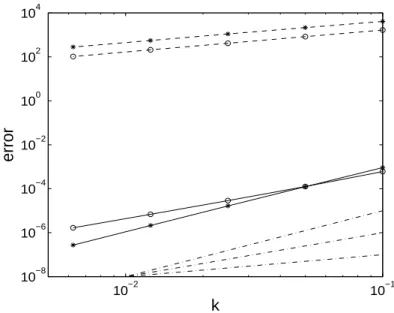
10−2 10−1 10−8
10−6 10−4 10−2 100 102 104
error
k
Figure 1: Local error (*) and global error (o) without avoiding (discont.) and avoiding (cont.) order reduction when integrating problem (40) with trapezoidal Lawson rule, (dash-dotted lines: slopes 1, 2 and 3),h= 2.5×10⁻³,k = 0.1,0.05, . . .
Local error order without avoiding O. R. 0.93 0.96 0.98 0.99 Local error order avoiding O. R. 2.88 2.92 2.95 2.96 Global error order without avoiding O. R. 1.00 1.00 1.00 1.00 Global error order avoiding O. R. 2.26 2.13 2.06 2.03
Table 2: Order corresponding to the integration of problem (40), with quadratic finite elements in space and trapezoidal Lawson rule in time,h= 2.5×10⁻³,k = 0.1,0.05, . . .
whose exact solution is u(x, t) = ex−t. For the space discretization, we have used
when-10−2 10−1 10−8
10−6 10−4 10−2 100
error
k
Figure 2: Local error (*) and global error (o) without avoiding (discont.) and avoiding (cont.) order reduction when integrating problem (41) with trapezoidal Lawson rule (dash-dotted lines: slopes 1, 2 and 3),h= 2.5×10⁻³,k = 0.1,0.05, . . .
Local error order without avoiding O. R. 1.13 1.21 1.23 1.24 1.25 Local error order avoiding O. R. 2.98 2.99 2.99 3.00 3.00 Global error order without avoiding O. R. 1.22 1.24 1.25 1.25 1.26 Global error order avoiding O. R. 2.37 2.19 2.09 2.05 2.02
Table 3: Order corresponding to the integration of problem (41), with quadratic finite elements in space and trapezoidal Lawson rule in time,h= 2.5×10⁻³,k = 0.1,0.05, . . .
everhdiminishes. (See Table 1.) However, with the technique suggested in this paper, we achieve to integrate the problem in an accurate way and, what’s more, avoiding completely order reduction. That can be observed in the slope of lines of Figure 1 and also in Table 2, where the precise values of the order (estimated from consecutive values of the error) are written. This corroborates Theorems 11 and 12 since order 3 for the local error and order 2 for the global one is observed.
In the second place, we have considered the vanishing boundary value problem
ut(x, t) = uxx(x, t) + (x2−x+ 2)e−t, x∈[0,1], t >0,
u(0, t) = u(1, t) = 0, (41)
whose exact solution is u(x, t) =x(1−x)e−t. We have discretized it in the same way
The second and fourth line of the table corroborate Theorems 11 and 12 because order 3 for the local error and order 2 for the global one are observed when order reduction is avoided. This means a significant improvement in contrast with the order 1.25 which is observed for the local and global errors without avoiding order reduction, as it was justified in [4].
5.3
Example 2. Finite-difference schemes
The finite-difference case can also be analysed under the framework in Section 4.1. Now, we can consider X = C(Ω) and Y = C(∂Ω). Besides, for each parameter h, we can consider a grid Ωh with some interior nodes in the interior of Ω and some
boundary nodes in ∂Ω. Associated to each Ωh, we can think of {Xh} as any finite
dimensional family of subspaces of X such that there is a one-to-one correspondence between each element of Xh and its nodal values in Ωh. The interior nodal values
determine the element in Xh,0 (for which the nodal values on the boundary vanish) while the boundary ones do the same inXh,b (for which the nodal values in the interior
vanish). The corresponding norm inXh will be the discreteL2-norm. We will consider
the interpolating operator Qh : Y → Xh,b, which takes any g ∈ Y to the function in
Xh,b whose nodal values on the boundary of Ωh coincide with those of g. Then, the
restriction of the operator Ah : Xh → Xh,0 (which approximates A) to Xh,0 will be represented by a certain square matrix, which we will denote asBh,0.
5.3.1 1-dimensional problem
We will firstly discretize problem (40) in space with the classical symmetric second-order FD scheme for the second derivative. For the discretization of the
wxx(x) =f(x), x∈(0,1), w(0) =w0, w(1) =w1,
this can be written as
Bh,0Wh,0+Eh[w0w1]T =fh,0,
where Wh,0 is the vector which contains the searched interior grid nodal values of w,
fh,0 is the vector which contains the interior grid nodal values off and
Bh,0 = 1 h2
−2 1 0 1 −2 1 . .. 0 1 −2 . .. 0
. .. ... ... 1 0 1 −2
, Eh
[ w0 w1 ] = 1 h2 w0 0 .. . 0 w1 .
In such a way, using the framework in (25), Rhw is represented by Wh,0, Bh,0 is the matrix which represents Ah,0 and Eh is the one which represents AhQh, Lh is just
the inside nodal projection and therefore, in this case, LhQh ≡ 0, which implies that
10−3 10−2 10−6
10−4 10−2 100 102 104
CPU time
error
Figure 3: Global error against cpu time when integrating (40) with trapezoidal Lawson quadrature rule without avoiding order reduction (dashed line), avoiding order reduc-tion (continuous line) and with the exponential quadrature rule (44) (dash-dotted line),
h = 2.5×10⁻³, k = 0.1,0.05, . . .. (Implementation calculating exponential-type ma-trices once and for all at the very beginning.)
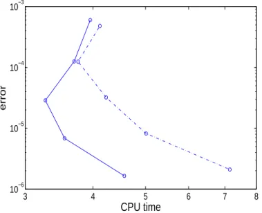
3 4 5 6 7 8
10−6 10−5 10−4 10−3
CPU time
error
and (23) and (24) in (H2) are clear. On the other hand, (H3) is also well-known to be satisfied withZ =H4(0,1) and ϵh =O(h2∥w∥H4(0,1)).
Notice that, in this particular case, when integrating in time with trapezoidal Law-son rule using the implementation in (31), the following scheme turns up:
Uh,n+1 = ekAh,0[Uh,n+
k
2Phf(tn)] +
k
2Phf(tn+1) +kφ1(kAh,0)AhQh∂[u(tn) +
k
2f(tn)]
+k2φ2(kAh,0)AhQh∂[Au(tn) +
k
2Af(tn)] +k 3φ
3(kAh,0)AhQh∂A2u(tn).(42)
Therefore, the only terms which must be calculated, apart from those which appear when applying trapezoidal Lawson method without avoiding order reduction to a van-ishing boundary conditions problem, are, forj = 1,2,
kj
h2φj(kBh,0)
Aj−1u(0, t
n) + k2Aj−1f(0, tn)
0 .. . 0
Aj−1u(1, t
n) + k2Aj−1f(1, tn)
, k 3
h2φ3(kBh,0)
A2u(0, t
n)
0 .. . 0
A2u(1, t
n) . (43)
When the stepsize is fixed, as we assume in our analysis, what is just required is then to calculate the first and last column ofφj(kBh,0) (j = 1,2,3) once and for all at the very beginning, and then at each step just the corresponding linear combination of those two columns must be performed. As distinct, all columns ofekBh,0 should be calculated
since, in principle, Uh,n and Phf(tn) have no vanishing components. Because of that,
the cost of computing (43) is negligible compared with that of calculating the first term in (42).
The global discrete L2-errors have been calculated without avoiding and avoiding order reduction. The results against CPU time when integrating till time t = 1 are shown in Figure 3. The time required to calculate the exponential-type matrices has not been considered since those calculations are performed just at the very beginning, and the relative cost of that part would very much depend on the final time of integration. The values ofk and hwhich have been considered are the same as in Figure 1 and, as the error in space is negligible with respect to that in time, the values for the errors are practically the same as in that figure. It is clear that, for each value ofk, avoiding order reduction implies a big reduction on the size of the error but a very small increase in computational time. Moreover, although it is not an aim of the paper to recommend any particular method, we have compared the results with the exponential quadrature rule which is based on interpolatingF in (11) by a linear polynomial. When integrating (21) with the mentioned rule and the above space discretization, for whichLhQh ≡0,
the scheme is given by
Uh,n+1 = ekAh,0Uh,n+kφ1(kAh,0)[AhQhg(tn) +Phf(tn)]
+kφ2(kAh,0))[AhQh(g(tn+1)−g(tn)) +Phf(tn+1)−Phf(tn)]. (44)
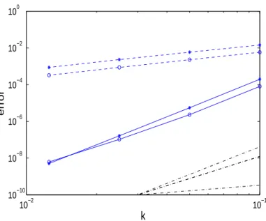
10−2 10−1 10−10
10−8 10−6 10−4 10−2 100
k
error
Figure 5: Local error (*) and global error (o) without avoiding (discont.) and avoid-ing (cont.) order reduction when integratavoid-ing problem (45) with vanishavoid-ing boundary conditions with Lawson Simpson rule (dash-dotted lines: slopes 1, 4 and 5), h=0.01, k=0.1,0.05,. . .
conditions problem. However, as it can also be observed in Figure 3, it is approximately twice more expensive than trapezoidal Lawson rule in this problem. The reason for that is that φ1(kBh,0) and φ2(kBh,0) must be calculated over full non-zero vectors. Notice that, if the number of stages with other exponential methods had to be in-creased to achieve a higher stiff order, the comparison would be even more beneficial for the implementation of Lawson methods as suggested here since the classical order is obtained without increasing the number of stages.
On the other hand, we have also made the numerical comparison between both second-order methods calculating the actions of the exponential-type matrices over vectors through Krylov techniques. In such a way, it is not necessary to calculate the exponential-type matrices at the very beginning, and the procedure could also be applied with variable stepsizes. For that, we have used the subroutines in [13] with the default values for the parameters in them. Figure 4 shows the results that we have obtained. At least for that problem, for the smallest values of k, the technique described here to implement the trapezoidal Lawson method is a bit cheaper than the mentioned exponential quadrature rule.
5.3.2 2-dimensional problems
results. The problem is
ut(t, x, y) = uxx(t, x, y) +uyy(t, x, y) +f(t, x, y), t >0, (x, y)∈Ω = (0,1)×(0,1),
u(t, x, y) = g(t, x, y), (x, y)∈∂Ω, (45)
with functionsf(t, x, y) and g(t, x, y) such that the exact solutions are
u(t, x, y) =x(1−x)y(1−y)ex+y−t and u(t, x, y) = ex+y−t.
For the space discretization of the Laplacian, we have considered the well-known fourth-order nine-point formula [19] while for the time integration we have used Lawson method based on Simpson’s quadrature rule, which is also of fourth order for prob-lem (9). More precisely, the scheme for the discretization of the Laplacian in a square,
wxx(x, y) +wyy(x, y) =f(x, y), ∂w=g in ∂Ω,
can be written (in terms of the searched nodal values in the interior Wh,0, the given
values ofg on the boundarywh,b and the values off in the interior and boundary grid
nodesfh,0 and fh,b) as
ChWh,0+Dhwh,b =Mhfh,0+Nhfh,b, (46)
whereCh and Mh are the tridiagonal block matrices
Ch =
1 h2 −10 3I+
2 3J
2 3I +
1
6J 0 . . . 0
2 3I+
1
6J − 10
3 I+ 2
3J . .. ... 0 . .. . .. . .. 0
..
. . .. . .. 23I+ 16J
0 . . . 0 23I+ 16J −103I +23J , (47)
Mh =
1 12
8I+J I 0 . . . 0
I 8I+J . .. ...
0 . .. . .. ... 0 ..
. . .. ... I
0 . . . 0 I 8I+J
, (48) with J =
0 1 0 . . . 0
1 0 1 ...
0 . .. ... ... ... ..
. . .. ... 1 0 . . . 0 1 0
,
and Dh, Nh correspond respectively to the associated block-matrices in Ch and Mh
acting on the boundary. This can be written as
Local error order without avoiding O. R. 1.29 1.34 1.41 Local error order avoiding O. R. 5.17 5.07 5.01 Global error order without avoiding O. R. 1.36 1.38 1.43 Global error order avoiding O. R. 5.11 4.47 4.09
Table 4: Order corresponding to the integration of problem (45) with vanishing bound-ary conditions, with nine-point formula in space and Simpson Lawson rule in time,
h= 0.01, k = 0.1,0.05, . . .
which resembles (25), whereBh,0 =Mh−1Ch represents the discretization Ah,0 and the operator Lh, when applied to the function f is represented by fh,0+Mh−1Nhfh,b. In
such a way,Phf =Lhf−LhQhf is represented by the interior nodal values off (fh,0). From the form of the matrices Ch and Mh (47)-(48), it is easy to see that both
matrices are symmetric and commute. Because of this, they diagonallize in the same base of eigenvectors. Applying Gerschgorin theorem, the eigenvalues ofCh are negative
and those ofMh are positive. Therefore, the eigenvalues ofBh,0 =Mh−1Ch are negative,
which implies (H1) withM = 1. On the other hand, (24) in (H2) is clear for γh = 1.
Besides, because of the fact that the eigenvalues of Mh are in (13,1) by Gerschgorin
theorem, the Euclidean norm ofMh−1 (which is symmetric) is bounded by 3. If we add to that the boundedness of the coefficients of Nh, (23) in (H2) follows. Finally, from
[19],
Chwh,0+Dhwh,b =Mhfh,0+Nhfh,b+O(h4∥w∥H6(Ω)),
where wh,0 is the vector which represents Phw and has the interior nodal values of w.
Subtracting from (46) and bounding in the corresponding norm,
∥wh,0−Wh,0∥=O(h4∥w∥H6(Ω)∥C−1 h ∥).
(Notice thath2C
hcan be written as the Kronecker product 16(4I+J)⊗(4I+J)−6Iand,
as the eigenvalues of J are {2 cos(2πj/N)}j=1,...,N−1 with N such that N h equals the side of the square, the eigenvalues ofh2C
h are{16(4+2 cos(2πj/N))(4+2 cos(2πl/N))−
6}j,l=1,...,N−1. From this it is clear that the smallest in modulus of the eigenvalues is
O(h2) and therefore Ch−1 is bounded independently of h.) AsWh,0 is the vector which representsRhw, (26) in (H3) follows withZ =H6(Ω) and εh =O(h4).
Again the local and global discreteL2-errors have been calculated for the vanishing boundary conditions problem without avoiding and avoiding order reduction. The re-sults when using a uniform grid space withh= 0.01 and time stepsizesk = 0.1,0.05, . . .