NUMERICAL SIMULATION OF THE VOCAL TRACT ACOUSTICS USING THE TLM METHOD

NUMERICAL SIMULATION OF THE VOCAL TRACT ACOUSTICS USING THE

TLM METHOD

PACS: 43.58.Ta; 43.70.Bk

Pelorson, Xavier1 ; Badin, Pierre1 ; Saguet, Pierre2 ; El Masri, Samir1 1

Institut de la Communication Parlée

UMR CNRS Q 5009, INPG, Université Stendhal. 46, avenue F. Viallet

F-38031 Grenoble Cedex 01 France

Tel: +33 4 76 57 45 36 Fax: +33 4 76 57 47 10

E-mail: [email protected], [email protected] 2

Laboratoire d'Electromagnétisme Microondes et Optoélectronique UMR CNRS 5530, INPG-UJF

23, Rue des Martyrs 38016 Grenoble Cedex 1 Tel: +33 4.76.85.60.13 Fax: +33 4.76.85.60.80 E-mail : [email protected]

ABSTRACT

The TLM method, originally developed for electromagnetism applications, has been adapted to simulate the acoustics of the vocal tract. Although the TLM method cannot overcome traditional techniques such as FEM or FDM in terms of computational costs, it is shown that this method can be a very useful and simple tool for acoustical investigations. Specific examples concerning the effects of a bend in the vocal tract, of the teeth or of 3-D propagation will be presented and discussed.

INTRODUCTION

Numerical tools are now widely used in speech acoustics research. While most popular techniques are based on the Finite Element Method (FEM) or the Finite Difference Method [1], [2], we present here an original method based on the Transmission Line Matrix Method (TLM). This method, originally developed for electromagnetism purposes [3] can indeed be applied to linear acoustical propagation thanks to the similarity between the equations of propagation of acoustic and electromagnetic waves. After a brief description of the method itself some specific simulation examples are presented.

THE BASICS OF THE TLM METHOD

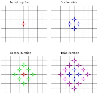
Principle of the Method

Fig 1: Illustration of the propagation and the scattering of pulses in a two-dimensional network.

Using the inductance, L and the capacitance, C of the transmission line, one can show that the equation of propagation for the voltage variation over a branch, Vy is [4]:

0

3

2

=

∂

∂

−

∆

t

V

LC

V

Which a classic linear propagation equation, similar to an acoustical one:

0

1

2 2

2

∂

=

∂

−

∆

t

P

c

P

where P is the acoustical pressure and c the sound velocity. Using adequate value for L and C (so that c = 1/(3LC)½) there is thus a direct analogy between the acoustical pressure P and the voltage variation Vy. In the same way, it can be show that a similar analogy can be obtained between the intensity current through the network and the acoustical particle velocity.

Boundary conditions

Since the TLM method is a time domain simulation method, boundary conditions require a specific treatment. Classical (frequency domain) approaches using impedance description of the boundaries are not applicable here. In order to ensure that the scattered pulses come back at a node in synchrony with the initial incident pulses, the boundaries must be placed at equal distance from adjacent nodes. For the sake of simplicity, in this paper, the vocal tract will be considered as hard walled.

Validation of the Method

The TLM method applied to the acoustics has been systematically validated by comparing the simulations with analytical solutions of classical problems, with measurements on in-vitro models of the vocal tract or by comparison with FEM simulations. A detailed description about these tests can be found in [5], [6].

VOCAL TRACT SIMULATION RESULTS

Simulation of the whole vocal tract

In the following we present simulation results obtained using three dimensional vocal tract geometries. These geometries were obtained from MRI data. The first examples present the simulation results obtained for the fricative /sh/. The geometry used is represented in Figure 2.

Sound source

glottis

lips

Fig. 2 : 3-D representation of the vocal tract for the sound /sh/

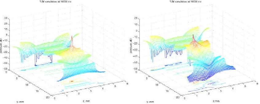
Two examples of simulation results are presented in Figure 3. In the first case, the sound source, a monopole, is placed on the centerline of the vocal tract structure. In the second case the sound source is placed near the wall of the vocal tract.

This example quite clearly enhances the crucial importance of the position of the sound source within the vocal tract. The spectacular differences observed between the two simulations can be explained in terms of higher transverse acoustical modes. It can been shown, indeed, that since 10 kHz is quite above the cut-on frequency of the first acoustical mode of this geometry a transverse mode can therefore propagate. However, a centred source cannot excite odd modes and, indeed, only plane waves (equal pressure contours are straight lines) are observed. On the opposite, in the case where the sound source is placed near a wall (which is more likely for a fricative), the first transverse mode is excited and propagates. As a result the radiated sound field is clearly asymmetrical (directivity effect).

Simulation of portions of the vocal tract

Global simulations of the vocal tract although often illustrative can sometimes lead to results that are difficult to interpret. This is the case when the geometry is so complex that it is not easy to evaluate which physical parameter is responsible for which variations. For this reason we used TLM simulations on isolated vocal tract structures in order to evaluate their acoustical consequences.

Simulation of a bent vocal tract

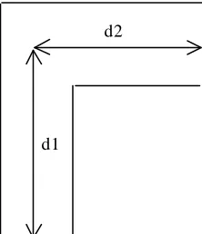
The first example deals with the effects of a 90° bend in the vocal tract.

Fig. 4: Simulation of a 90° bend of the vocal tract.

On table 1, we present an example of comparison between the resonance frequencies obtained using the TLM simulation with those obtained by neglecting the bend and assuming an equivalent uniform pipe of length d1+d2.

Equivalent uniform vocal tract TLM simulations of a Bend

1376 1320

2669 2940

3957 4120

4463 4610

5040 5290

Table 1: Comparison between the resonance frequencies, in Hz, of a 90° bent vocal tract and a uniform straight one

As can be seen from this example, the differences are less than 10 % which is small enough to neglect the effects of the curvature of the vocal tract. This result supports the conclusion already stated by Sondhi [7].

Simulation of the teeth d1

The last example deals with the even more complex configuration depicted in figure 5. Such configuration would thus, crudely, represent the obstacle formed by the teeth.

Fig. 5: geometry of an obstacle formed by the teeth. All dimensions are in mm.

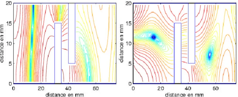
Two examples of results are presented in Figure 6.

Fig. 6: Pressure contours in the (x-y) plane simulated using TLM method. Left curve at 6kHz, right curve at 8 kHz.

As can be seen from Figure 6, strong acoustical perturbation are observed due to the presence of the teeth. These effects and the way to account for them, as an end correction, is curently under investigation.

CONCLUSION

Although it certainly can't rivals traditional FEM/FDM packages in terms of flexibility or in terms of computing costs (memory loads, computing speed), the TLM method has proven itself to be a quite useful tool for "simple" linear acoustics problems such as those encountered in speech research.

BIBLIOGRAPHICAL REFERENCES

[1] Lu C., Nakai T., Suzuki H. (1993) "Finite element simulation of sound transmission in the vocal tract", J. Acoust. Soc. Jpn., 14, 63-72.

[2] Matsuzaki H;, Miki N., Ogawa Y. (1996) "FEM analysis of sound wave propagation in the vocal tract with 3-D radiational model", J. Acoust. Soc. Jpn., 17, 163-166.

[3] Johns P.B, R.L. Beurle, (1971) "Numerical solution of 2-dimensional scattering problems using a transmission line matrix", Proc. IEE, 118, 1203-1208.

[4] Saguet P. (1985). "Analyse des milieux guidés la méthode MTLM", Doctorat d’Etat , Institut Nationale Polytechnique de Grenoble

[5] Elmasri S., Pelorson X., Saguet P., Badin P. (1998)" The use of the Transmisson Line Matrix in acoustics and in Speech", International Journal of Numerical Modelling, 11, 133-151.

[6] El-Masri S.D. (1997). "Application de la méthode numérique TLM ( Transmission Line Matrix ) aux ondes acoustiques et à la parole", thèse de doctorat de l’Institut Nationale Polytechnique de Grenoble.

[7] Sondhi M. M. (1986) "Resonances of a bent vocal tract", J. Acoust. Soc. Am., 79, 1113-1116.

ACKNOWLEDGEMENTS