Economic growth, consumption and oil scarcity in Colombia : A Ramsey model, time series and panel data approach

,661

%RUUDGRUHVGHO&,(

&HQWURGH,QYHVWLJDFLRQHV(FRQyPLFDV 8QLYHUVLGDGGH$QWLRTXLD

&HQWURGH,QYHVWLJDFLRQHV(FRQyPLFDV

8QLYHUVLGDGGH$QWLRTXLD

0HGHOOtQ&RORPELD

La serie Borradores del CIE está conformada por documentos de carácter provisional en los que se presentan avances de proyectos y actividades de investigación, con miras a su publicación posterior en revistas o libros nacionales o internacionales. El contenido de los Borradores es responsabilidad de los autores y no compromete a la institución

1ƒ

0DU]RGH

(FRQRPLF*URZWK&RQVXPSWLRQ

DQG2LO6FDUFLW\LQ&RORPELD

$5DPVH\PRGHOWLPHVHULHVDQGSDQHOGDWDDSSURDFK

Elaborado por:

Danny García Callejas

(&2120,&*52:7+&2168037,21$1'2,/6&$5&,7<,1&2/20%,$ $5$06(<02'(/7,0(6(5,(6$1'3$1(/'$7$$3352$&+

Danny García Callejas1

5HVXPHQ este artículo muestra la relación que existe entre el crecimiento económico, del

consumo y de la disponibilidad de petróleo en Colombia. Primero se realiza un análisis

teórico modificando el modelo de crecimiento de Ramsey para incluir una variable que

represente la disponibilidad de petróleo, llegando a la conclusión que la tasa de crecimiento

del consumo está directamente relacionada con la tasa de crecimiento de la producción de

petróleo. Luego, por medio de un modelo de series de tiempo y panel de datos se verifica

este resultado teórico y se muestra que la disponibilidad de petróleo contribuye al menos en

un 13% en la tasa de crecimiento económico de Colombia.

3DODEUDV FODYHconsumo, crecimiento económico, escasez, reservas y producción de

petróleo.

$EVWUDFW this paper shows the existing relation between economic growth, consumption

and oil availability growth rate in Colombia. Firstly a theoretical analysis using a modified

Ramsey growth model in which a variable that represents oil availability is performed,

concluding that consumption’s growth rate is directly related with oil production growth

rate. Later, this theoretical result is verified using a time series and panel data analysis

which shows that oil availability provides at least a 13% of Colombia’s economic growth.

.H\ZRUGVconsumption, economic growth, scarcity, oil production and reserves.

-(/FODVVLILFDWLRQQ01, Q32, Q38, Q43.

1

Professor of the Economics Department at the University of Antioquia —Medellín, Colombia— and member of the Enviromental Economics Research Group —GEMA, for its Spanish abbreviation— at the Economics Research Center —CIE, for its Spanish abbreviation— at the same university.

,QWURGXFWLRQ

The Ramsey (1928), Harrod (1939) Domar (1946) and Solow (1956) Swan growth

models represent economist’s concerns about economic growth and their possible

determinants, however, new difficulties and the importance of natural resources on growth

generate new questions that should be answered and that can still be analyzed using their

theoretical approaches. This paper takes advantage of the Ramsey (1928) growth model and

modifies it to include a non-renewable resource as oil. After solving the model an

interpreting its outcomes, the main conclusion is that consumption growth rate is directly

related with oil production growth rate or oil reserves, that is, if an economy has oil scarcity

and cannot obtain it from other sources, for example imports or input substitution, then its

future consumption can be jeopardized.

The economic data and statistics on oil, consumption and economic growth present a

direct association that entails Latin America to have a constant source of this input. Even

though this region possesses important reserves the amount they demand is also high and

according to Jones (2003) this estimate of reserves could exceed the true available quantity.

Such a situation would put Latin-American countries in a complicated position that would

require, in order to surpass it, substitutes of this input or other energy sources different from

those provided by oil. This paper evidences through a panel data and time series analysis

that a reduction in oil availability could reduce Colombia’s growth rate in at least 13%.

Developing countries have been demanding more oil and require it every time more and

more. According to Gately and Streifel (1997) world oil demand in the 1971 – 1993 period

has increased in 18.3 million barrels per day and for that increase developing countries are

the most responsible since they participated with 14.2 million barrels per day from the

quoted increase. Therefore, future research must not be disregarded because developing

countries like Latin-American ones require more oil every year and the effects of oil shocks

on these economies and the microeconomic effects and between sector impacts of this

possible situation using a general equilibrium frame should be studied.

This paper is divided in three sections: firstly an interpretation of statistic and

descriptive data using bar and time series graphs is made; secondly a modified Ramsey

economic interpretation will be encountered. Thirdly, an empirical approach using time

series and panel data analysis that proves the theoretical and model’s statements is

presented. Finally, the most relevant conclusions and references used in this paper will be

detailed.

,2LODVD6FDUFH5HVRXUFH

The planet can run out of oil in any moment because the available quantity of oil on

earth is practically fixed and reserves are lesser than expected (Jones, 2003). Oil is

produced by the earth, but its renewal rate is very low and near to zero making it a

non-renewable resource but current extraction levels will not allow oil to renew, therefore it will

disappear. “As geologists make clear, there is an embarrassingly limited amount of

conventional oil in the earth’s crust, and it is QRW wise to suppose that these assets can be

greatly augmented” (Banks, 1997, p. 2).

Even if it is thought that the fixed quantity is very big and high oil sector productivity

will save us (Rauch, 2001), it can be quoted that “Although some economists still find it

possible to claim that oil is inexhaustible, geological authorities are increasingly expressing

the belief that this resource is painfully finite in an economic sense, because eventually it

might become too costly to produce in amounts supplied earlier” (Banks, 1997, p. 1), and

this shows how the production, of this resource, will have to decline in some moment of

time.

As Graph 1 illustrates, the Colombian case will not be as different as the one predicted

by the theory and the results of the modified Ramsey Model in section 2. This South

American country might see its consumption possibilities reduced in the future if it does not

search for a commodity that substitutes its oil needs or if new reserves are not discovered.

Graph 1 warns on this possibility: there is a positive relation between consumption and oil

reserves, therefore if oil reserves reduce consumption will follow the same pattern; this idea

will be confirmed through the time series and panel data econometric models.

*UDSK. Colombia: Oil Reserves and Consumption, 1950-1995

0 500 1.000 1.500 2.000 2.500 3.000 3.500 4.000

0 100.000 200.000 300.000 400.000 500.000 600.000 700.000 Oil reserves versus consupmtion Polinómica (Oil reserves versus consupmtion)

6RXUFH: Autor’s calculation. Ecopetrol (2004), DNP (2004) and Dane (2004).

The concerning problem is that duration of oil reserves in Colombia have been

diminishing in an important way. Graph 2 shows this tendency that seems to sustain in the

long run. This problem is not despicable since it could generate a consumption and

production abridgement. As Halvorsen and Smith (1986) show, the possibility of reducing

the effects that the scarcity of a natural resource can cause on the economy is through a

substitute that does not have a high price. The problem is that a high price of a natural

resource can be a signal of its depletion (Hotelling, 1931), nevertheless, this could appear

only towards the end of its exhaustion what does not allow this variable to control demand

and secure its future availability (Reynolds, 2004).

*UDSK. Colombia: Oil Reserves Useful Life

0 5 10 15 20 25 30 35 40

1950195219541956195819601962196419661968197019721974197619781980 198219841986198819901992 1994 Year

Y

ea

rs

Reserves useful life Lineal (Reserves useful life)

The Latin American and World economies are oil dependant. As graphs 3 and 4 present,

there is a positive relation between production and oil energy use. Modern economies can

not move without fuel that is why oil price increases affect economic growth and can even

generate recessions, they are simple too oil dependant (Irons, 2000). Recessions will bring

low income and thus will add consumption abridgement worsening the situation and

obliging economies to find cheaper and more reliable energy alternatives.

*UDSK. Latin America: GDP at 1995 Prices and Energy produced

from Oil (kt of oil), 1971-2001

700.000.000.000 900.000.000.000 1.100.000.000.000 1.300.000.000.000 1.500.000.000.000 1.700.000.000.000 1.900.000.000.000 2.100.000.000.000

0 100.000 200.000 300.000 400.000 500.000 600.000 700.000 Latin America’s Energy Oil Use (kt of oil)

L

at

in

A

m

er

ic

a’

s

G

D

P

Latin America Energy produced from oil and GDP, at 1995 prices Lineal (Latin America Energy produced from oil and GDP, at 1995 prices)

6RXUFH: Author’s calculations. World Bank (2004).

*UDSK. Earth: GDP at 1995 prices and Energy Oil Use (kt of oil), 1971-2001

10.000.000.000.000 15.000.000.000.000 20.000.000.000.000 25.000.000.000.000 30.000.000.000.000 35.000.000.000.000

0 2.000.000 4.000.000 6.000.000 8.000.000 10.000.000 12.000.000 World Energy Oil Use (kt of oil)

W

o

rl

d

G

D

P

World GDP and Energy Oil Use, at 1995 prices Lineal (World GDP and Energy Oil Use, at 1995 prices)

25.000

20.000

15.000

10.000

5.000

0

-5.000

-10.000 25.000

20.000

15.000

10.000

5.000

0

-5.000

-10.000

Japan Middle

East

Africa FSU NAFTA

Other Asia*

China Latin

America Europe

Production Net exports

The Latin American case discloses a positive relation between GDP production and

energy production since the later is an important input of the former. The outlook is far

worse than expected. Latin-American reserves account for almost 10% of worldwide oil

availability and according to a recent —2003— study made by Sweden’s Uppsala

University, oil reserves are at least 80% lesser than predicted and production levels will

peak in the next ten years (Jones, 2003).

*UDSK. Share of World Crude Oil Reserves and Production by Region

6RXUFH: Carvahlo and Suni (2002, p. 56).

The Latin-American and Colombian scenario worsen when the net exports are

examined in Graph 6, not only the region does not have a high reserve level but it is

increasingly importing crude oil and in the near future will become a net importer that will

depend directly on its international providers that do not have as much as it was thought

(Jones, 2003). As Olson (1988) arguments, oil shocks can aggravate GDP recessions,

contribute to diminish productivity and generate macroeconomic instability, problems that

can exacerbate distribution and poverty problems in the region.

*UDSK. Crude Oil Production and Net Exports in Selected Regions, 1000 barrils per day

6RXUFH: Carvahlo and Suni (2002, p. 56).

%

60

50

40

30

20

10 0

NAFTA

%

60

50

40

30

20

10

0 Other Asia*

Latin America

Europe FSU Middle East Africa China Japan Production

Japan Other Pacific

Asia 90

80

70

60

50

40

30

20

10

0

Mexico Canada Others Latin USA Australia Europe China World Africa

America

90

80

70

60

50

40

30

20

10

0

The dependency on Middle East Crude Oil is a key factor that can bring difficulties for

all economies in the future. In 2000 40.2% of the World’s total oil supply was met by the

Organization of Petroleum Exporting Countries —OPEC— (Perry, 2001) and in 2003 the

Middle East —which includes part of the OPEC members— produced 30% of the World’s

consumption (Esser, 2004). Graph 7 shows a difficult prospect for Japan which imports

from the Middle East more than 80% of the oil it requires. Even though Latin America

appears to be in the last places in this category, it does need to import at least 25% from this

Arab region. The problem is that reserves are estimated to hold until 2050 or, in the best

scenario, until 2080 (Vozza, 2003), situation that will bring yield complications and

generate incentives to countries intensive in oil as an input to search for a substitute.

*UDSK. Dependency on Middle East crude oil in selected regions,

share in total oil imports, in percentage

6RXUFH: Carvahlo and Suni (2002, p. 56).

Perhaps one of the alternatives is international commerce and the discovery of new

reserves that will satisfy world oil demands —improbable according to Jones (2003)—.

The first one will reduce recession possibilities of Developing countries only if they can

trade with big oil producers and not find that these only sell to Developed countries as

Lawrence and Levy (1982) show. If price does correct demand due to resource

exhaustibility as Hotelling (1931) explains then the risk of a major crash appears to be real

if there are no available substitutes. That impossibility of price to correct demand is more

plausible than Hotelling’s (1931) idea (Aldeman, 1990, p. 9) since price can rise at a high

point when agents think that the resource is scarce but as it is exploited and demand

increases its price elevates lesser. Krautkraemer (1998, pp. 2066) also exhibits how in the

,,5DPVH\¶V*URZWK0RGHODQG2LO

Ramsey’s growth model was developed in 1928 and, since then, it has been applied to

different economical situations. In this case, we will apply such model to the oil sector in

order to try to establish the theoretical relation between oil supply’s growth and economical

growth. The idea, then, is to see the long run consequences on growth of oil supply

changes; for this a Ramsey model with oil as a natural resource that generates utility to

economic agents will be introduced in order to determine the new variable’s consequences

to growth.

We will assume that this economy produces two goods: the first one is a “generic” good

that can be consumed or saved and that only requires of capital (K) and labor (L) to be

supplied; the second one will be oil (P) that is only available in a fixed quantity, therefore,

it is treated as a non-renewable resource. We will also assume that economical agents have

a utility function in which they include these two goods from which they obtain satisfaction

when they are consumed (C). This economy’s production pattern will be represented

through a Cobb Douglas production function (1).2

Y = F(K, L) = Akβ (1)

Utility hill have positive but diminishing marginal utility returns (2).

U’(c, p) > 0 y U’’(c, p) < 0. (2)

It will also be assumed that this economy has a population that represents entirely its

labor force that grows at a fixed rate called Q. We can describe the mass of workers at any

moment in time by the equation L = ent, where Wrepresents the different periods of this

economy.

The agent’s utility function in this economy will be the combination of the proposed

function by Cash and Koopmans and the utility function that agents would have if the only

good in the economy were oil. The latter is going to be an exponential function like this

one: Pα, where α< 1 is a parameter. Hence, supposing that these two functions can be

united in one that is using the separability and adding-up properties, then the following

expression can be obtained:

2

α θ

θ

=F−

F

8 (3)

In this way, the consumption side of this economy has been showed, however, agents

can save their goods and this is essential in the economy’s growth because it will be

through savings that capital will grow and, therefore, production. This is observed in

equation (1) where production has a positive relation with capital’s per capita amount. In

consequence, the condition for capital growth is given by:

. & / . ) W

.( ) = ( , )− −δ (4)

Thus, it is clear that the economy’s problem is to maximize economical agent’s utility

subject to their saving capacity but taking in account the depreciation rate (δ) because

the latter is the principal long run growth cause; and, they are aware, specially

policymakers, of the positive capital growth influence and the initial capital stock k(0) > 0.

Since these agents are rational, they will search to get the highest utility as possible so they

solve the following problem:

∫

Max.8 F F H ✁ GW

ρ α θ

θ

r. NW = $Nβ −F− Q+δ N− ₍₅₎

As observed, this is a dynamical optimization problem; for solving it, Hamilton’s

maximizing method will be used in order to establish the optimum growth path. But that θ,

the inverse intertemporal substitution elasticity, is greater than zero must be kept in mind

and that ρ > n represents the temporal preference parameter. Thus, knowing the fixed

values of equation (5), Hamilton’s method in order to optimize utility is used; this is given

by the following expression:

) p ) ( ( P 1 1 ) , , p , ( ( ) 1 − + − − +       +       − −

= F − _H− − _{$N F Q N}

N F + ✂ ✄ δ λ θ λ θ α ρ β (6)

From equation (6) the equations for the maximum’s principle that are key in

determining the maximum values of the variables will be obtained; then following

equations will appear:

0 ) ( c

H ₌ ( ) _{− =}

∂ ∂ − − − W H F ☎ ✆

λ

H _{-1 ( )}

= − =

∂

∂ _H− − ✝ _W

✞

λ

α α ρ

) ( )) ( )( ( k H 1 W Q $N

W

β

δ

λ

λ

= ∂

∂ −

(9)

Taking logarithm to equations (7) and (8), deriving respect to time and having in mind

equation (9) the following two equations that solve this maximization problem will be

acquired:3 ) ( 1 ) ( )

(

β

ρ

δ

θ

p β 1 ρ δ

α

β _{− −}

− −

= _$N −

W W

(11)

But, it must be taken in account that in the long run the economy will tend to the steady

state and in this period of time the aggregated variable’s growth is fixed and per capita’s

variables growth is none, therefore, from equations (10) and (11) can be concluded that in

such moment, the following must be true:

) ( p ) ( p ) ( ) ( W W W F W F ₌

(12)

Equation (12) shows a direct relation between consumption growth rate and oil production

growth rate or reserves. An economy that does not have the sufficient oil to attend its needs

and to use as an input in its production process will have difficulties in increasing its

consumption patterns because production will be jeopardize due to the unavailability of an

important resource —oil— and due to this income will not grow and therefore consumption

possibilities will be abridged.

,,,'DWDDQGUHVXOWV

Using information gathered by Dane (2004), DNP (2004) and Ecopetrol (2004),4 a time

series and panel data analysis was performed in order to establish the veracity of the

conclusions proposed by the theoretical model in Section II and described through

statistical indicators in Section I, that is, it will be shown that growth and consumption have

a direct pattern with oil availability and production.

3

For more details on the model’s mathematical development please refer to Appendix A.

4

Firstly, a time series analysis will be developed. In order to do such analysis the first step

according to Enders (1995) is to check if the variables are stationary, that is if they do not

have a unit root. In doing so, two unit root tests are applied for the logarithmic variables.

The statistics of the Philips Perron and Augmented Dickey Fuller tests are shown in Table

1.

7DEOHColombia:Augmented Dickey Fuller and Philips Perron

Unit Root Tests, 1950 – 1995

9DULDEOH $XJPHQWHG'LFNH\)XOOHU 3KLOLSV3HUURQ

Statistic Critical Value Statistic Critical Value

*'3DWSULFHOHYHO Level

1st Difference

0.569881 -3.784810 -3.5162b -3.5189b 0.812558 -3.266357 -3.1854c -3.1868c , &RQVXPSWLRQDW SULFHOHYHO Level 1st Difference

-0.545829 -3.237905 -3.1868c -3.1898c -0.745764 -5.248398 -4.1728a -4.1781a , &DSLWDODWSULFHOHYHO Level

1st Difference

-0.882294 2.026386

-1.9483b -1.9486b

6.666018 -3.5814a

,

(FRQRPLFDOO\DFWLYH SRSXODWLRQ

Level 1st Difference

1.967797 3.082803

-2.6182a -2.6196a

29.27399 -2.6143a

,

$FFXPXODWHGRLO SURGXFWLRQ Level 1st Difference

1.881455 2.009950

-1.9514b -1.9492b

12.28847 -2.6143a

,

$QQXDORLOSURGXFWLRQ Level

1st Difference

-0.387507 -3.677514 -3.5348b -3.5162b 0.063431 -4.191675 -3.5112b -3.5136b , $QQXDORLOUHVHUYHV Level

1st Difference

-0.502108 -4.551428 -4.1781a -4.1837a -0.532772 -7.270790 -4.1728a -4.1781a , 5HVHUYHVXVHIXOOLIH Level

1st Difference

-2.073557 -4.870828

-4.1781a -4.1837 a

-2.679154 -6.019963

-4.1728a -4.1781a

,

For the Augmented Dickey Fuller test, the Durbin Watson was always near or equal to two as the test requires it.

a, b, c correspond to 1%, 5% and 10% rejection levels.

The theoretical model analyzed in Section I, specifically in Equation 12, proposes a direct

relation between consumption and oil production growth rates indicating that the

econometric model should not be estimated in level but using a differenced form. This

the differenced variables —first difference. Consequently a differenced translog model was

estimated including capital, labor force and accumulated oil production as a proxy of oil

exhaustibility. Since the differenced variables did not have a unit root, a cointegration

analysis was not required nor using second difference variables. The theoretical model

pointed a direct relation between differenced variables, therefore, if a cointegration analysis

would be to be met the differenced variables —first difference— must have a unit root

recommending as shown by Enders (1995, p. 219) an estimation of a second difference

model or a cointegration process.

Most papers that have estimated production functions use Cobb-Douglas functional forms,5

however, as Greene (2000, p. 217) points out this is a nested model that should be

estimated only after proving a hypothesis test that sustains that the Translog model can be

reduced to a Cobb-Douglas form. The Translog functional form relating GDP growth —Y,

labor —L— and accumulated production of oil or oil exhaustibility —P— and including a

constant term — 0— and a proxy for technological progress or time trend —T— can be

expressed econometrically as:

lnY = 0 + 1lnK + 2lnL + 3lnP + 4(lnK)2 + 5(lnL)2 + 6(lnP)2 + 7(lnK)(lnL)

+ _{8(lnK)(lnP) + 9(lnL)(lnP) + 10T + t}

(13)

The results of estimating the Differenced Translog model using data for the period

1951-1995 —45 observations— and performed through Least Squares is presented in Table 2.

However estimation results were not satisfactory since capital presented a negative relation

with GDP growth which is against neoclassical growth functions theoretical proposition but

resulted to be not significant indicating that it is highly probable that its value is zero. Oil

exhaustibility did not result significant nor two of the three interactions involved in the

regression. These outcomes can be evidence of an inadequate functional form advising that

the Cobb-Douglas model could be an admissible form.

5

7DEOH.Colombia:Estimating a Differenced Translog Model

with Stationary Variables, 1950 – 1995

'HSHQGDQWYDULDEOH&RORPELD¶V*'3JURZWKUDWH

9DULDEOH &RHIILFLHQW 9DULDEOH &RHIILFLHQW

Capital growth rate -0.232667 (-0.101589)

0.5 * Capital growth rate * Accumulated oil production growth rate

54.15918 (1.084017) Capital growth rate squared -11.64963

(-0.967802)

0.5 * Capital growth rate * Economically active population growth rate

40.74926 (0.355626) Accumulated oil production

growth rate

6.836699 (1.363128)

0.5 * Accumulated oil production growth rate * Economically active population growth rateb

-390.5678 (-1.984131) Accumulated oil production

growth rate squared

-14.47131 (-0.563804)

Constantb -0.567482

(-1.847754) Economically active population

growth ratea

26.42297 (2.220786)

Trendb -0.000668

(-1.961823) Economically active population

growth rate squareda

-248.9895 (-2.247359)

R-squared 0.485404 Durbin-Watson statistic 1.841908

Adjusted R-squared 0.334052 F-statistic 3.207126

a, b are significant at 5% and 10% respectively. T-Statistics in parenthesis.

Due to the results in Table 1 and the suspicion of a nested model, specifically a

Cobb-Douglas, a Wald Coefficient test was performed. The results are presented in Table 3 and

clearly show the viability and adequacy of estimating a Cobb-Douglas with the variables

included in the prior econometric analysis. Its functional form would be:

lnY = 0 + 1lnK + 2lnL + 3lnP + 107 t

(14)

7DEOHWald Test for Coefficient Equality: Proving if the Translog Model

can be treated as a Cobb-Douglas

1XOO+\SRWKHVLV 4 = 0 5 = 0 6 = 0 7 = 0 8 = 0 9 = 0

F-statistic 1.118729 Probability 0.372226 Chi-square 6.712373 Probability 0.348268

Thanks to the results achieved with the Wald coefficient test in Table 2, the Cobb-Douglas

functional form is validated and estimated in Table 3. Outcomes are satisfactory and

predicted by theory and other growth production related papers like Douglas (1976).

Dornbusch, Fisher and Startz (2002, p. 47) find that labor is three times more important

than capital in U. S. production after estimating a Cobb-Douglas. In this case —Table 4—

labor force growth rate represents almost five times the growth rate that capital can

experiment and which would contribute to GDP growth, nevertheless, a oil exhaustibility is

a variable that is not included in regular production function analysis subtracting weight or

importance to capital since oil can be accounted as an input required by capital goods in

tasks such as the production of energy for the economy or in industrial processes. So if

capital growth rate and accumulated oil production growth rate are united labor force

growth rate will answer for more than double of the GDP’s growth rate adjusting more to

other papers conclusions.

7DEOH. Colombia: Cobb Douglas Model, 1950 – 1995

'HSHQGDQWYDULDEOH&RORPELD¶V*'3JURZWKUDWH

9DULDEOH &RHIILFLHQW

Capital growth rate 0.461745 (2.643312) Accumulated oil

production growth rate

0.551862 (2.905878) Economically active

population growth rate

2.391183 (4.211328)

Constant -0.053178

(-2.360238)

Trend -0.000805

(-3.234322)

R-squared 0.383811

Adjusted R-squared 0.322192 Durbin-Watson statistic 1.854780 F-statistic 6.228790 T-Statistics in parenthesis.

All variables in Table 4 are significant and additional tests that are presented in Appendix 3

show the model’s reliability. But, what does this result mean? Firstly it shows that GDP

growth is positively impacted by oil availability so if oil exhaustibility comes to happen the

import oil and search for energy substitutes and the former will only be possible if there are

still world reserves or if those reserves where to be sold to Colombia because developed

nations would compete for this input and would have the upper hand card in the deal; the

latter, a technological improvement or substitute, would be possible if enough research and

development is done by private and public entities but this requires a state policy for this

matter that is not available in Colombia because government and private resource must be

dedicated to more important and urgent issues; therefore the only possibility is that such

technology or oil substitutes becomes available on the world market and Colombia has the

resources for buying it. This important resource and its availability should not be despised

since it accounts for 13% or more Colombia’s growth rate, according to the econometric

model and by adding up all the other effects and dividing the impact of oil by this sum.

The reduction in oil availability clearly affects an oil dependant economy like Colombia,

but would this affect consumption as predicted by the theoretical model proposed in

Section 1? The answer is yes and this should be clear theoretically. If production reduces so

does income and if that happens consumption will be abridged also due to lower revenue.

Empirically, a differenced Cobb-Douglas is estimated having as dependant variable

consumption growth rate and including oil exhaustibility and a proxy of technology. The

signs and results that appear in Table 5 are as expected and show the direct relation

between oil accumulated production growth rate and technology; indeed, if technology

improves then the possibility of oil substitutes is more possible, however, the first impact

caused by oil is much higher than technology specially when no research and development

are made in this field.

7DEOH. Colombia: Consumption and Resource Availability estimated

with a Differenced Cobb Douglas, 1950 – 1995

'HSHQGDQWYDULDEOH&RORPELD¶VFRQVXPSWLRQJURZWKUDWH

9DULDEOH &RHIILFLHQW

Oil accumulated production growth ratea

0.713802 (5.887904)

Trendb 0.000380

(1.706178)

R-squared 0.154518

Adjusted R-squared 0.116150 Durbin-Watson statistic 1.760608

F-statistic 59.17940

a, b significant at 1% and 10%. T-Statistics in parenthesis.

Even though theprior analysis satisfies the theoretical backgrounds from which it is taken,

the data availability on oil production and consumption in each region —state— is

sufficient for a panel data approach. Can there be differences among states and time that

cannot be perceived with the time series analysis and that can affect seriously our

conclusions? The best way to answer this question is through panel data. This methodology

gives the possibility of controlling non-observed heterogeneity invariant in time. In this

case we cannot observe the efficiency with which each region produces, its need for oil and

machines that work with this input, their substitution capacity between resources and their

geographical conditions for obtaining oil from their terrain or producing energy by means

different to oil sources. These reasons entice a panel data analysis specified as follows:

cit =

✟

✠✡

[ + i + it, i = 1, …, 16 and t = 1, …, 10 (15)

Where cit represents consumption growth rate, GDP growth rate or GDP per capita growth

rate; xit constitute the characteristics of each region —state— that can include invariant

columns in time, and specifically, will be composed by oil production growth rate and oil

production growth rate squared or oil accumulated production growth rate and oil

accumulated production growth rate squared and a time trend that represents technology

In order to avoid panel data spurious regressions in the above suggested model, Baltagi

(2001) suggests applying at least one panel data unit root test. In this case, the variables

included in the panel data will be tested with the Im Pesaran Shin (1997) and Levin Lin

Chu (2002) tests. The null hypothesis in these tests is that each series in the panel contains a

unit root (H0 i = 1, for all i) and the alternative is that at least one of the series is

stationary (H1 i < 1, for at least one i); the results, that all variables are stationary or that

reject the null hypothesis, are presented in Table 6.

7DEOH.Colombia:Im Pesaran Shin and Levin Lin Chu Unit Root Tests

for variables from 16 regions, 1991 – 2001

,P3HVDUDQ6KLQ /HYLQ/LQ&KX

9DULDEOH 7VWDWLVLWLFIRU

WHVWLQJ+☛ ☞

&RQFOXVLRQ 7VWDWLVLWLFIRU WHVWLQJ+☛ ☞

&RQFOXVLRQ

Accumulated oil production growth rate -3.367 Reject H0 -12.181 Reject H0

Annual oil production growth rate -3.247 Reject H0 -10.980 Reject H0

Consumption growth rate -2.822 Reject H0 -10.865 Reject H0

GDP growth rate -2.790 Reject H0 -10.908 Reject H0

GDP SHUFDSLWD growth rate -2.565 Reject H0 -10.515 Reject H0

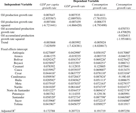
After confirming that all variables are stationary, a panel data analysis was made and

presented in Table 7. Four fixed effects models were estimated, after making checking with

different panel data models —between, population averaged and random effects, the best

results are presented only. Different intercepts were dealt with and in the four cases a

marginal decreasing returns of scale are encountered showing that oil exhaustibility has an

important impact at the beginning but the effect’s growth diminishes each time allowing to

infer that even though this energy resource is important its losing relevance in the long run.

This could be related with additional energy resources that these regions possess like

hydroelectric plants, coal plants and the use of other inputs different from oil or the

possibility of substituting this need with other resources or having the advantage of

producing good and services that do not heavily require oil and its derivatives.

7DEOHColombia:Panel data estimations with different intercepts relating GDP and per

capita’s growth rate and consumption’s growth rate with oil exhaustibility

for 16 regions, 1991 – 2001

'HSHQGDQW9DULDEOH ,QGHSHQGHQW9DULDEOH *'3SHUFDSLWD

JURZWKUDWH *'3JURZWKUDWH

&RQVXPSWLRQ JURZWKUDWH

&RQVXPSWLRQ JURZWKUDWH

Oil production growth rate 0.007647 (2.855567)

0.007535 (2.889703)

0.014411 (7.781553) Oil production growth rate

squared

-0.007484 (-6.721441)

-0.007439 (-6.866420)

-0.006375 (-8.793490) Oil accumulated production

growth rate

0.070753 (4.470829) Oil accumulated production

growth rate squared

-0.026411 (-1.951681)

Trend -0.003868

-7.025059

-0.003992 (-7.424381)

-0.005024 (-8.020817) Fixed effects intercept

Antioquia 0.027089a 0.042990a 0.058192a 0.017080a Arauca -0.061275 -0.019235 -0.003735 -0.046722

Bolívar 0.029242b 0.054374a 0.069226a 0.027042a

Boyacá 0.025892b 0.033391a 0.048251a 0.006712

Casanaré 0.078392 0.112935 0.125805 0.075841 Cauca 0.035992b 0.053935a 0.069007a 0.013475 Cesar 0.044416a 0.063775a 0.078110a 0.033104a Cundimarca 0.050936a 0.072843a 0.087824a -9.19E-05

Huila 0.020582a 0.036562a 0.051113a 0.008675 Meta 0.037910a 0.057835a 0.072163a 0.027937a Nariño 0.041020a 0.061444a 0.074719a 0.024371b Norte de Santander 0.031227a 0.054473a 0.069431a 0.027376a Putumayo 0.083762 0.114355 0.129138 0.085991 Santander 0.058520a 0.072734a 0.087798a 0.046580a Sucre 0.033968a 0.054090a 0.072215a 0.016000b Tolima 0.041967a 0.045675a 0.058927a 0.011917

Adjusted R2 0.172788 0.207721 0.191719 0.097258

a, b, c represent intercepts significant at a 1%, 5% and 10% respectively. T-Statistics in parenthesis.

Table 8 presents the result of estimating the fixed effects model with a common intercept

providing similar outcomes to the ones appearing in Table 7. A positive but marginal

decreasing relation is disclosed as in the above estimation, nevertheless, the positive

relation between GDP growth rate, GDP per capita growth rate and consumption growth

rate and oil exhaustibility concerns since reserves might disappear before than expected

(Jones, 2003); regions, therefore, should entice policies that orient their economy towards

its derivates. Public transport and private car owners should use and adopt more efficient

vehicles that require less gallons of fuel per mile or that run on fuels not derived from oil.

7DEOHColombia:Panel data estimations with common intercept relating GDP and per

capita’s growth rate and consumption’s growth rate with oil exhaustibility

for 16 regions, 1991 – 2001

'HSHQGDQWYDULDEOH ,QGHSHQGHQW9DULDEOH GDP per capita

growth rate GDP growth rate

Consumption growth rate

Consumption growth rate

Oil production growth rate 0.008240 (3.185754)

0.007355 (2.983831)

0.014453 (7.047456) Oil production growth rate

squared

-0.005865 (-6.103572)

-0.005345 (-5.861186)

-0.004453 (-6.754321) Oil accumulated

production growth rate

0.082945 (3.977070) Oil accumulated

production growth rate squared

-0.042468 (-2.244263)

Trend -0.003789

(-6.910835)

-0.003956 (-7.327766)

-0.004678 (-7.653015) Common intercept 0.034304

(10.31101)

0.053362 (16.41124)

0.066629 (16.25258)

0.021169 (5.408523)

Adjusted R2 0.127140 0.187675 0.197181 0.126222

T-Statistics in parenthesis.

&RQFOXVLRQV

Oil is a scarce resource that will last shorter than expected (Jones, 2003) and Colombia, as

many other countries, depends on this resource as an input, energy source and export

product. Such is the dependency that production and energy provided by oil are directly

related and output requires the latter in order to yield goods and services. The problem is

that the region consumes a great part of its oil production but, in the future, will have to

import from other countries specially those from the Middle East because Latin America’s

reserves are below this regions amount.

Scarcity becomes a problem because the whole world depends on oil in order to move and

generate energy and high prices do not appear as constraints for oil consumption as

Hotelling (1931) predicted because the uncertainty in the exact reserves amount and the

exports show a difficult scenario for Latin American countries. Also if the impossibility to

pay as much for oil as developed nations and their negotiation power is added, it will be

found, as shown by Lawrence and Levy (1982) that developed countries have the upper

hand and first option for buying this scarce resource so countries as Colombia will have to

wait and see if they can import at least a fraction of this black gold.

The econometric analysis using a time series and panel data approach both confirm for

Colombia a positive relation between GDP growth, consumption growth and oil

exhaustibility. The first method uses the idea of a neoclassical production function that

allows encountering the importance of oil in production, concluding that this scarce

resource contributes for at least 13% of output growth. Therefore, if Colombia’s oil

reserves do not satisfy national demand and imports become difficult to obtain, growth will

be affected and production and energy generation through this fossil fuel will be at risk.

This problem might be met in the near future because Colombia’s reserves useful life

present a diminishing tendency. The second approach confirms this result for Colombian

regions but conveys a better scenario where oil dependency, in the long run, is abridged and

its impact is lesser every time.

Future research should be oriented to determine the impact of oil scarcity at a

microeconomic level and determining the best market organization and produce output that

gives the optimum response to oil shocks and that allows the economy to minimize oil

shocks. This would require analyzing specific sectors and their interrelations, ideas that

would be better treated with a general equilibrium model for the regional and national

5HIHUHQFHV

Adelman, M. A., 1990. “Mineral Depletion, with Special Referente to Petroleum”, 7KH

5HYLHZRI(FRQRPLFVDQG6WDWLVLWLFV, 72, 1, pp. 1-10.

Azofeifa, Ana Georgina; Villanueva, Marlene, 1996. “Estimación de una función de producción: caso de Costa Rica” [internet paper], Banco Central de Costa Rica, http://www.bccr.fi.cr/ndie/Documentos/PI-06-1995-R-ESTIMACION%20DE%20UN A%20FUNCION%20DE%20PRODUCCION.PDF. Access: august 12th 2004.

Banks, Ferdinand, 1997. “Economic Theory and the Supply of Oil”, :RUNLQJ 3DSHU

8SSVDOD8QLYHUVLW\, 22.

BARRO, Robert; SALA-I-MARTIN, Xavier. (FRQRPLF*URZWK, McGraw Hill, 1995.

Carvahlo, Anthony de; Suni, Paavo, 2002. “War, Oil and Economic Growth” [internet

paper], The Resaearch Institutute of Finnish Economy, )(6, 4,

www.etla.fi/files/913_FES_02_4_war_oil.pdf, pp. 52-62

Colombia, Departamento Nacional de Planeación —DNP—, 2004. “Series históricas”, [internet data base], DNP, http://www.dnp.gov.co/03_PROD/PUBLIC/1p_ee.asp. Access: august 12th 2004.

Colombia, Departamento Administrativo Nacional de Estadística —Dane—, 2004.

“Estadísticas para Colombia” [internet data base], Dane, http://www.dane.gov.co. Access: august 12th 2004.

Colombia, Empresa Colombiana de Petroleos —Ecopetrol—, 2004, “Estadísticas de la industria”, [internet data base], Ecopetrol, http://www.ecopetrol.com.co. Access: august 12th 2004.

Douglas, Paul, 1976. “The Cobb-Douglas Production Function Once Again: Its History, Its Testing, and Some New Empirical Values”, 7KH -RXUQDORI3ROLWLFDO(FRQRP\, 84, 5, pp. 903-916.

Domar, Evsey, 1946. “Capital Expansion, Rate of Growth, and Employment”,

(FRQRPHWULFD, 14, 2, pp. 137-147.

Enders, Walter, 1995. $SSOLHG(FRQRPHWULF7LPH6HULHV, New York, John Wiley and Sons.

Esser, Charles, 2004. “Brief Non-OPEC fact sheet” [internet paper],

http://www.eia.doe.gov/emeu/cabs/nonopec.html . Access: august 12th 2004.

Gately, Dermot; Streifel, Shane, 1997. “The Demand for Oil Products in Developing

Countries”, :RUOG%DQN:RUNLQJ3DSHU, 359.

Greene, William H., 2000. (FRQRPHWULF$QDO\VLV, New Jersey, Prentice Hall.

Halvorsen, Robert; Smith, Tim, 1986. “Substitution Possibilities for Unpriced Natural Resources: Restricted Cost Functions for the Metal Mining Industry”, 7KH 5HYLHZ RI (FRQRPLFVDQG6WDWLVWLFV, 68, 3, pp. 398 – 405.

Harrod, Sir Roy, 1939. “An Essay in Dynamic Theory”, (FRQRPLF-RXUQDO, 49, pp. 14-33. Hotelling, Harold, 1931. “The Economics of Exhaustible Resources”. -RXUQDORI3ROLWLFDO (FRQRP\. 39, 2, pp. 137 - 175.

Im, K. S., Pesaran, M. H. and Y. Shin. “Testing for Unit Roots in Heterogeneous Panels”

-RXUQDORI(FRQRPHWULFV July 2003, 115(1); pp. 53-74.

Jones, Graham, 2003. “World Oil and Gas Running Out” [internet paper], CNN

International World, http://edition.cnn.com/2003/WORLD/europe/10/02/global.

warming/, Access: august 13th of 2004.

Krautkraemer, J. A. 1998. “Nonrenewable resource scarcity”. -RXUQDO RI (FRQRPLF

Lawrence, Colin; Levy, Victor, 1982. “On Sharing the Gains from International Trade: The Political Economy of Oil Consuming Nations and Oil Producing Nations”,

,QWHUQDWLRQDO(FRQRPLF5HYLHZ, 23, 3, pp. 711-721.

Levin, Andrew; Chien-FuLin; and Chia-Shang J. Chu. “Unit Root Tests in Panel Data:

Asymptotic and Finite-Sample Properties” -RXUQDO RI (FRQRPHWULFV, May 2002,

108(1); pp. 1-24.

Olson, Mancur, 1988. “The Productivity Slowdown, The Oil Shocks, and the Real Cycle”,

7KH-RXUQDORI(FRQRPLF3HUVSHFWLYHV, 2, 4, pp. 43-69.

Perry, George, 2001. “The War on Terrorism, the World Oil Market and the U.S. Economy” [internet paper], Analysis Paper, 7, http://www.brook.edu/views/papers/ perry/20011024.htm. Access: august 12th of 2004.

Ramsey, Frank P., 1928. “A Mathematical Theory of Saving”, (FRQRPLF-RXUQDO, 38, 152,

pp. 543-559.

Rauch, Jonathan. “The New Old Economy: Oil, Computers, and the Reinvention of the

Earth”, [internet paper], The Atlantic Online, January 2001,

http://www.theatlantic.com/issues/2001/01/rauch.htm. Access: February 24th of 2002. Reynolds, Douglas, 2004. “The Mineral Economy: How Prices and Costs Can Falsely

Signal Decreasing Scarcity” [internet paper], http://www.hubbertpeak.com/reynolds/

MineralEconomy.htm. Access: February 24th of 2004.

Solow, Robert M., 1956. “A Contribution to the Theory of Economic Growth”, 4XDUWHUO\

-RXUQDORI(FRQRPLFV, 70, pp. 65-94.

Vozza, Tyson, 2003. “OPEC’s Role in Future Development: Increased Investments for Domestic Economic Growth and Increased Aid for Poor Developing Countries”

[internet paper], http://www.stanford.edu/class/e297c/OPEC's%20Role%20in%20

$SSHQGL[$Expansion of the Theoretical Model

Below the necessary steps for obtaining equation 10 will be described. For this purpose,

equations 7 and 9 will be used.

0 ) ( c

H ₌ ( ) _{− =} ∂

∂ _F− _H− − ✌ _W

✍

λ

ρ θ

ln(c−θe− ( ρ− n ) t = ln(λ (t))

−θ ln c − (ρ− n) t = ln(λ (t))

t )) ( (ln t t) n)) ( c) ln (( ∂ ∂ = ∂ − − −

∂ θ ρ λ W

• • = + − − λ λ ρ

θ n ( )

c(t) c(t) W n ) ( 1 c(t)

c(t) _{=− + +}

• • ρ λ λ θ W

And from 9, λ(t)/λ can be obtained and replacing it in the above equation and adding up

terms it can be disclosed:

)) ( ( 1 c(t) c(t) ₁ δ β θ β − + = − • Q $N

In a similar way equation 11 can be demonstrated but, for doing so, equations 8 and 9 are

$SSHQGL[%Descriptive Statistics of the Variables Used in the Econometric Analysis

7DEOH%Descriptive Statistics

Variable Mean Standard Deviation

GDP at 1975 constant prices

405,228.53 233,742.87

Consumption at 1975 constant prices

288,656.70 158,806.70

Capital at 1975 constant prices

1,162,072.77 684,607.80

Economically active population

8,004,960.23 3,363,439.44

Accumulated oil production

1,834.27 959.63

Annual oil production 77.14 44.73

Oil reserves 1,179.76 741.80

Borradores del CIE

1R 7tWXOR $XWRUHV )HFKD

01 Organismos reguladores del sistema de saludo colombiano: conformación, funcionamiento y responsabilidades.

Durfari Velandia Naranjo Jairo Restrepo Zea Sandra Rodríguez Acosta

Agosto de 2002

02 Economía y relaciones sexuales: un modelo económico, su verificación empírica y posibles recomendaciones para disminuir los casos de sida.

Marcela Montoya Múnera Danny García Callejas

Noviembre de 2002

03 Un modelo RSDAIDS para las

importaciones de madera de Estados Unidos y sus implicaciones para Colombia

Mauricio Alviar Ramírez Medardo Restrepo Patiño Santiago Gallón Gómez

Noviembre de 2002

04 Determinantes de la deserción estudiantil en la Universidad de Antioquia

Johanna Vásquez Velásquez Elkin Castaño Vélez

Santiago Gallón Gómez Karoll Gómez Portilla

Julio de 2003

05 Producción académica en Economía

de la Salud en Colombia, 1980-2002

Karem Espinosa Echavarría Jairo Humberto Restrepo Zea Sandra Rodríguez Acosta

Agosto de 2003

06 Las relaciones del desarrollo económico con la geografía y el territorio: una revisión.

Jorge Lotero Contreras Septiembre de 2003

07 La ética de los estudiantes frente a los exámenes académicos: un problema relacionado con beneficios

económicos y probabilidades

Danny García Callejas Noviembre de 2003

08 Impactos monetarios e institucionales de la deuda pública en Colombia 1840-1890

Angela Milena Rojas R. Febrero de 2004

09 Institucionalidad e incentivos en la educación básica y media en Colombia

David Fernando Tobón Germán Darío Valencia Danny García

Guillermo Pérez

Gustavo Adolfo Castillo

Febrero de 2004

10 Selección adversa en el régimen contributivo de salud: el caso de la EPS de Susalud

Johanna Vásquez Velásquez Karoll Gómez Portilla

Marzo de 2004

11 Diseño y experiencia de la regulación en salud en Colombia

Jairo Humberto Restrepo Zea Sandra Rodríguez Acosta

Marzo de 2004

12 Economic Growth, Consumption and

Oil Scarcity in Colombia: A Ramsey model, time series and panel data approach

Danny García Callejas Marzo de 2005

&HQWURGH,QYHVWLJDFLRQHV(FRQyPLFDV )DFXOWDGGH&LHQFLDV(FRQyPLFDV 8QLYHUVLGDGGH$QWLRTXLD

&RUUHRHOHFWUyQLFRFLH#DJXVWLQLDQRVXGHDHGXFR 7HO7HO)D[

$$