SOME CASES OF CROSSOVER BEHAVIOR IN HEART INTERBEAT AND ELECTROSEISMIC TIME SERIES

c

World Scientific Publishing Company

Articles

SOME CASES OF CROSSOVER BEHAVIOR

IN HEART INTERBEAT AND

ELECTROSEISMIC TIME SERIES

A. MU ˜NOZ-DIOSDADO

Unidad Profesional Interdisciplinaria de Biotecnolog´ıa, Instituto Polit´ecnico,Nacional Av. Acueducto s/n,L. Ticom´an,M´exico, D. F. 07340, M´exico

[email protected]

L. GUZM ´AN-VARGAS

Unidad Profesional Interdisciplinaria en Ingenier´ıa y Tecnolog´ıas Avanzadas Instituto Polit´ecnico Nacional, Av. IPN No. 2580, L. Ticom´an

M´exico D. F. 07340, M´exico

A. RAM´IREZ-ROJAS

Departamento de Ciencias B´asicas, Universidad Aut´onoma Metropolitana Azcapotzalco, M´exico D. F., 02200, M´exico

J. L. DEL R´IO-CORREA

Universidad Auton´oma Metropolitana Iztapalapa M´exico D. F., 09340, M´exico

F. ANGULO-BROWN

Escuela Superior de F´ısica y Matem´aticas,Instituto Polit´ecnico Nacional Edif. No. 9, U. P. Zacatenco, M´exico D. F., 07738, M´exico

Received January 25, 2005 Accepted March 23, 2005

Abstract

Fractal time series with scaling properties expressed through power laws appear in many con-texts. These properties are very important from several viewpoints. For instance, they reveal the nature of the correlations present in the fractal signals. It is common that the scaling prop-erties characterized by means of invariant quantities suffer changes along with the dynamical

evolution of the studied systems. One of these changes is a crossover in the scaling properties reflecting an important change in the system dynamical behavior. In this article, we present two cases of crossover behavior corresponding to interbeat and electroseismic time series, we observe the crossovers in time series of experimental data and their corresponding simulation with simple models. We suggest a possible explanation of the observed crossovers in terms of the models considered.

Keywords: Fractal Dimension; Time Series; Multifractals; Heart Rate Dynamics; Crossover Behavior; Electroseismic Time Series.

1. INTRODUCTION

In recent years, the so-called fractal time series have received a lot of attention in many fields of sci-ence. In fractal fluctuating signals is common to find power law scaling behavior in several statisti-cal measures of the time series. Among the most usual methods for scaling studies of time series are the Hurst rescaled-ranged analysis,1 the power spectrum analysis,2 the detrended fluctuation anal-ysis (DFA)3,4 and the Higuchi fractal method.5,6 Two of the fields where those methods have been applied are both in some physiological signals7,8 as the heartbeat time series and in the so-called seismic electric signals (SES).9,10 _{In the first case,} the healthy heartbeat is traditionally thought to be regulated according to the principle of home-ostasis whereby physiological systems operate to reduce variability and achieve an equilibrium-like state.11 However, some recent studies12 show that even under resting conditions the human heartbeat fluctuations display the kind of long-range corre-lations typically exhibited by dynamical systems far from equilibrium.13 Nevertheless, in some cases, such as patients with severe congestive heart failure and healthy elderly subjects the long-range corre-lation behavior shows a breakdown manifested as a crossover phenomenon in some statistical mea-sure of the time series, such as, fractal dimen-sion D;8,14 DFA exponent α4,7 and the spectral exponentβ.15

In the case of SES, crossover phenomena have also been reported — which are possibly relevant for the question of discriminating between a true signal (SES activity) and an artificial noise.16 The solution of this question is considered a crucial test for the feasibility of the so-called VAN method for searching electric precursors of seisms.17 Rel-evant crossover phenomena in scaling properties have also been reported in the study of correla-tions in sea-level elevacorrela-tions of the North Sea;15 in

systems exhibiting continuous phase transitions;18 in particle flow through a single pore;19 in simpli-fied models of a limit order market20 and in jerky flows.21 In the present work, we study some inter-esting crossover phenomena occurring in both heart interbeat time series and SES arising from electric self-potentials measured in an electro-seismic sta-tion located at Guerrero state near the Mexican subduction zone.22 The article is organized as fol-lows. In Sec. 2, we introduce a brief resume of the four methods we use for the time series analysis (DFA, Higuchi method, power spectrum and multi-fractal analysis). In Sec. 3, we show the crossovers appearing in both cardiac and electroseismic series when they are analyzed by means of the methods of Sec. 2. In Sec. 4, we propose some numerical mod-els reproducing the crossover behavior observed in Sec. 2. Finally, in Sec. 5, we present some conclu-sions of our study.

2. METHODS

2.1. Spectral Method

A time series can be either described in the time domain asx(t) or in the frequency domain in terms of the amplitudeX(f, T) where f is the frequency. This amplitude can be calculated by means of the Fourier transform applied to x(t) in the interval 0< t < T.

X(f, T) =

_T

0 x(t)e

2πif t_{dt. (1)}

The quantity |X(f, t)|2df is the contribution to the total energy ofx(t) from those components with frequencies between f andf+df. The power spec-tral density is obtained by dividing by the period T, thus,

S(f) = 1

T|X(f, T)|

in the limit T → ∞. Then, the product S(f)df is the power in the time series associated with the fre-quency rangef andf +df.

A fractal property of a time series is reflected as a power law dependence between the spectral power and the frequency by means of an exponent, termed the spectral exponent

S(f)∼ 1

fβ. (3)

The value ofβ, is the slope of the best-fit straight line to log(S(f)) versus log(f) and is a measure of the strength of the persistence or anti-persistence in a time series.2 It is well known that the power spectrum can be considered as the Fourier cosine transform of the correlation function as is stated by the Weiner-Khintchine theorem.23 In this sense, also, the value of β is strongly related to the type of correlations present in a time series. For exam-ple, the uncorrelated white noise has a β ≈ 0, Brownian motion, the typical example of short cor-related noise has a β ≈ 2, and the 1/f noise, that exhibits long-range correlations, has β ≈ 1. For calculation purposes, it is more convenient to use a more efficient method as the well-known Fast Fourier Transform algorithm.

2.2. DFA Analysis

New methods arising from the nonlinear dynamics have been converted in important tools to obtain relevant information from physiological time series. In 1993, Peng et al.3 introduced a new method to detect long-range correlations called Detrended Fluctuation Analysis. This method is based in the classical random walk variations and has been used to detect long-range correlations in highly hetero-geneous DNA sequences and other physiological signals.3 To illustrate the DFA method we depart from an initial time series (of total lengthN), first, this series is integrated, y(k) =N_i=1[B(i)−Bave],

after this, the resulting series is divided into boxes of size n. In each box of length n, a straight line is fitted to the points, termed the local trend, yn(k). Next, the line points are subtracted from the inte-grated series y(k), in each box. The root mean square fluctuation of the integrated and detrended series is calculated by means of

F(n) =

1

N N

k=1

[y(k)−yn(k)]2. (4)

This process is taken over several scales (box sizes) to obtain a power law behavior between F(n) and nα, with α an exponent which reflects self-similar properties of the signal. The exponent α gives the information about the type of sig-nal, α = 0.5 corresponds to white noise (non-correlated signal), α = 1 means 1/f noise and α = 1.5 represents a Brownian motion. There exist also a well-known relationship betweenα and the spectral exponent β, α = (1 + β)/2.24 The DFA analysis has been used in the analysis of correlations of interbeat time series, for example, in 1996, Iyengar et al.24 suggested that aging is associated with disruption in the fractal-like long-range correlation that characterizes healthy sinus rhythm cardiac interval dynamics. They showed by means of DFA and spectral analysis that healthy young subjects have interbeat time series with fractal scaling expressed through a unique scaling exponent (in the case of DFA, α ≈ 1). On the other hand, in the case of healthy old individuals, the interbeat interval time series had two scal-ing regions, over the short range, interbeat inter-val fluctuations resembled a random walk process (α≈1.5) whereas over the long-range, they resem-bled white noise (α ≈ 0.5). According to Iyengar

et al.,24 this age-related loss of fractal organiza-tion (the pass of one exponent to two exponents) in heartbeat dynamics may reflect the degrada-tion of integrated physiological regulatory systems and may impair an individual’s ability to adapt to stress.

2.3. The Higuchi’s Method

Fractal dimension of self-similar objects in the plane is defined in terms of the isotropic distribution of their parts which can be scaled by a unique scale factor. This property changes in the case of self-affine fractals because their spatial distribution is not isotropic and the scaling factor is different for each direction. Higuchi5 proposed a method to cal-culate fractal dimension of self-similar curves in terms of the slope of a straight line that fits the length of the curve versus the time interval (the lag) in a double log plot. The method consists in considering a finite set of data taken at a regular interval,

From this series, we construct a new time series vmk, defined as

v(m), v(m+k), v(m+ 2k), . . . , v

m+

N−k k ·k

(6)

with m = 1,2,3, . . . , k, where [ ] denotes Gauss’s notation and k, m are integers that indicate the initial time and the interval time, respectively. The length of the curvevk

m, is defined as:

Lm(k) = 1 k      

[N−m k ]

i=1

|v(m+ik)

− v(m+ (i−1)k|

 

N_N−−_m1

k k    (7)

and the term N−1 [N−m

k ]k.k

represents a normalization

factor. Then, the length of the curve for the inter-val k, is given by L(k), the average value over k sets Lm(k). Finally, if

L(k) ∝k−D (8) then the curve is fractal with dimension D.5 For the case of self-affine curves, this fractal dimen-sion is related with the spectral exponent β by means of β = 5−2D, where if D is in the range 1 < D <2 then 1 < β < 3.5 Higuchi showed that this method provides an accurate estimation of the fractal dimension.

2.4. Multifractal Analysis

Multifractal structures have been found in a grow-ing number of physical problems. Recently, multi-fractal analysis has also been used for the study of physiological time series.11,25 For instance, Ivanov

et al.11 established the relevance of the multifrac-tal formalism for the description of a physiologi-cal signal. They stated that it is natural to expect a need for multifractal concepts to describe heart-beats since they are a result of the interaction of many physiological components operating in differ-ent scales. Therefore, the output of the signal has a nonlinear and inhomogeneous character.

Multifractal distributions are characterized by the function f(α), the fractal dimension, plotted against α, the H¨older exponent, or the multifrac-tal spectrum.11,26For the analysis of interbeat time series, we used the method proposed by Chhabra

and Jensen27,28 that provides a highly accurate, practical and efficient method for the direct com-putation of the singularity spectrum f(α). We can consider a time series as a singular measureP(x) if we normalize it. We calculate the f(α)-curve, first covering the measure with boxes of lengthL= 2−n and computing the probabilitiesPi(L) in each of the boxes. We then construct the one-parameter family of normalized measures with

µi(q, L) =

[Pi(L)]q

j

[Pj(L)]q.

(9)

Finally, for each value ofqwe evaluate the numer-ators on the right-hand-sides of the equations:

f(q) = lim L→0

i µi

(q, L) ln [µi(q, L)]

lnL (10)

α(q) = lim L→0

i

µi(q, L) ln [Pi(L)]

lnL (11)

for decreasing box sizes (increasingN). We extract f(q) and α(q) from the numerators slopes versus lnL. The parameter q provides a microscope for exploring different regions of the singular measure. For q >1,µ(q) amplifies the more singular regions of P, while for q < 1 it accentuates the less singu-lar regions, and forq= 1 the measure replicates the original measure. Equations (10) and (11) provide a relationship between a Haussdorf dimensionf and an average singularity strength α as implicit func-tions of the parameter q. The plot of f versus α is the multifractal spectrum. The mass exponent1 τ(q) is given in terms of the α(q) and the fractal dimensionf(α(q)) by

τ(q) =qα(q)−f(α(q)). (12)

The curvef(α) characterizes the measure and is equivalent to the sequence of mass exponentsτ(q). We can also describe the measure with the general-ized fractal dimensionsDq which are given by

Dq= τ (q)

1−q. (13)

3. OBSERVED CROSSOVERS

earthquakes occurring at a point where the dimen-sion of the event equals the down-dip width of the seismological layer (see Fig. 1 of Pacheco et al.29). Small earthquakes grow in both length (L) and width (W); their rupture dimensions have no bounds. On the other hand, large earthquakes, have no bounds in rupture length, but their down-dip width is limited by thickness of the region capable of generating earthquakes.29 Another phenomenon where dimensionality plays an important role in crossover behavior of power laws is the case of sea-level elevations, in the North Sea. Dimon et al.15

analyzed a 105-year time record of hourly sea-level elevations for the port of Esbjerg, Denmark. These authors calculated the power spectrum of this time series finding that, in addition to well-known peri-odic components, the power spectrum has a low-frequency broadband structure with three regimes behaving approximately as f0, f−1.2 and f−2.4 as frequency increases. They attributed this behav-ior to driven, damped Kelvin waves. The crossover to a nearly white noise spectrum occurs at fwn ∼ 5×10−7Hz ∼(20d)−1 (d is days). Above this fre-quency, there is a region where S(f)∼f−1.2 _(1/f -like noise) and at a frequency fc ∼ 5×10−6Hz ∼ (2d)−1, the spectrum crosses over rather sharply into a regime where S(f) ∼ f−2.4 underneath the lunar tidal peaks. Under a model based in the so-called telegraph equation, they interpret the crossover frequencyfcas that where the penetration depth of the waves is of the order of h (the unper-turbed water depth). At high frequencies the pene-tration depth is small and dissipation at the bottom is not important. At low frequencies the penetration

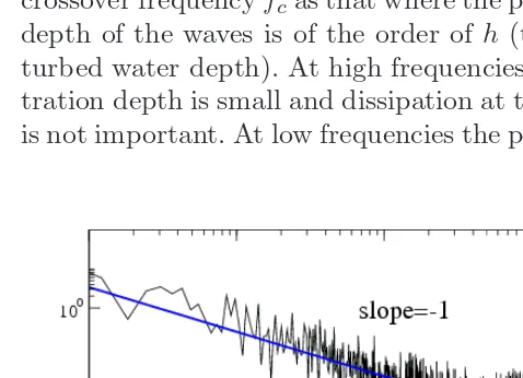
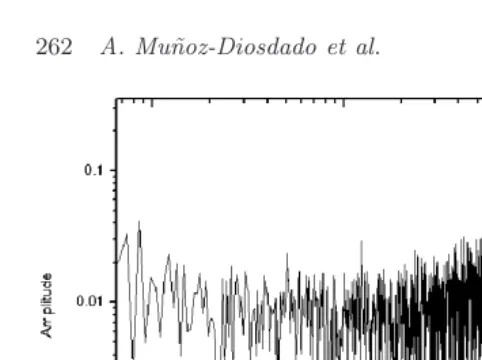
Fig. 1 The log-log ofS versusf of a healthy young indi-vidual (32 years old) displays a 1/f-like behavior.

depth becomes comparable to the depth, dissipa-tion becomes dominant, and waves can no longer propagate. That is, in the Dimon et al. model the role of the fc has a clear physical interpretation in terms of a change in water depths. Another case of crossover behavior in power law relationships is that reported by Berge et al.19 by means of a rescaled-range analysis and power spectra of particle flow trough a single pore. In their experiment (and sim-ulation), particles suspended in an electrolyte are caused to flow trough a pore by pressure difference. Each particle in the pore gives rise to a pulse in the measured pore resistance. The pulse height is pro-portional to the particle volume and the pulse width is given by the particle velocity. In dilute solutions, individual particle pulses can be detected and ana-lyzed, but at higher concentrations the pulses over-lap and the signal looks like noise. The signals were analyzed by Berge et al. by means of the Hurst’s exponent and the power spectrum and they find a clear crossover from persistent behavior for short times corresponding to the fact that particles reside a finite time in the pore to an independent process corresponding to the uncorrelated entry of particles into the pore.

Here, we focused our attention in the study of crossover phenomena occurring in two systems: (1) heart interbeat time series and (2) signals arising from electric self-potentials measured in an electro-seismic station near the Mexican subduction zone in the state of Guerrero.

we depict a typical log-log plot of the power spec-trum corresponding to a healthy young individual (32 years old) displaying an 1/f-like behavior. In Fig. 2, we show the power spectrum of a represen-tative healthy elderly subject (77 years old) with an evident crossover around f = 0.03. Both previ-ous time series were taken from Physionet31 corre-sponding to short segments of ECGs (two hours) equivalent to approximately 8000 beats.

The observed crossover power spectra can also be observed by means of both DFA analysis (Fig. 3) and the fractal Higuchi’s method (Fig. 4). We shall discuss this crossover behavior in the next section.

Between 1992 and 1998, the fluctuations of the electric self-potential of the ground in several sites

Fig. 2 The log-log ofS versusf of a healthy elderly indi-vidual (77 years old) has a crossover aroundf= 0.03 Hz.

Fig. 3 DFA plot of logF(n) versus logn for data from one elderly healthy subject (Fig. 2) and its simulation, the crossover is evident. The agreement between experimental and simulated data is reasonable.

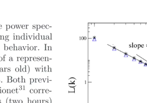
Fig. 4 Plot of logL(k) versus logk of heart interbeat sequences of the same data of Fig. 2. The crossover in both experimental and simulated data is also evident.

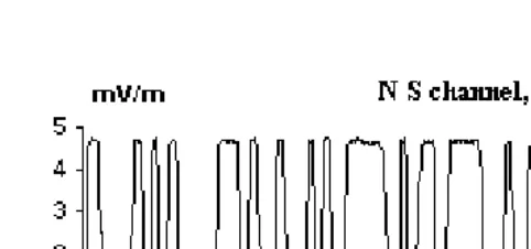
Fig. 5 Details observed in a short segment corresponding to NS channel monitored through an electroseismic station at Acapulco, Mexico.

Fig. 6 Details observed in a short segment corresponding to EW channel monitored in the station mentioned in Fig. 5.

Fig. 7 Representative power spectra behavior in the NS channel: white noise.

(August 1994–July 1996) we find several behaviors: white noise (Fig. 7), 1/f-like noise (Fig. 8) and evi-dent crossovers (Fig. 9). For a discussion on these different behaviors in relation to theMs = 7.4 EQ, see Ram´ırez-Rojaset al.32 When the electric signal file corresponding to Fig. 7 is analyzed by means of the DFA and the Higuchi’s method, we obtain Figs. 10 and 11 respectively, where the crossover phenomena are also evident.

Fig. 8 Representative power spectra behavior in the NS channel: 1/f-like behavior.

Fig. 9 Representative power spectra behavior in the NS channel: electroseismic crossover.

Fig. 11 The electroseismic crossover calculated by using the Higuchi method.

For the case of the multifractal analysis, the crossover behavior corresponding to Figs. 2 to 4 is depicted in Figs. 12 to 14. The multifractal spec-trum does not show the crossover in a clear way, but it differentiates the dynamics of the interbeat time series of young healthy persons and elderly healthy persons. This difference is displayed as a loss of mul-tifractality in the interbeat time series, it means that the width of the spectrum of elderly persons is small in comparison with the width of the spec-trum of young persons (Fig. 13). The narrow mul-tifractal spectrum for the elderly persons in Fig. 12

0.98 0.99 1 1.01 1.02 1.03 1.04 1.05 1.06 0.3

0.4 0.5 0.6 0.7 0.8 0.9 1

α

f(

α

)

* young

o old

Fig. 12 Multifractal spectra of real data (young healthy and elderly healthy subjects). Interbeat time series of healthy young subjects and their simulation (see Fig. 14) display a broad multifractal spectra whereas the series of elderly healthy subjects and their simulation (Fig. 14) show narrow spectra.

-30 -20 -10 0 10 20 30

0.985 0.99 0.995 1 1.005 1.01 1.015 1.02 1.025 1.03 1.035

q

Dq

o old

* young

Fig. 13 Spectrum of generalized fractal dimensionsDq as a function of the moment order q for real data (young and elderly healthy subjects).

0.940 0.96 0.98 1 1.02 1.04 1.06 1.08 1.1

0.1 0.2 0.3 0.4 0.5 0.6 0.7 0.8 0.9 1

α

f(

α

)

* young (simulated)

o old (simulated)

Fig. 14 Multifractal spectra of simulated data.

is reflected in the flat Dq spectrum in Fig. 13. It seems to be that a crossover is reflected as a change in the width of the multifractal spectrum.

4. SOME NUMERICAL MODELS

Recently, a simple model of the aging effect in heart interbeat time series was proposed.14 This model is based on combinations of noisy first-order autore-gressive series. A simple model of 1/f noise is a stochastic process composed of a superposition of many modes with different time constants.13 One time constant can be obtained from a single first-order autoregressive process,

Xt+τ+1=aXt−τ +εt−τ (14)

where ε is a Gaussian distributed random variable and a is a coefficient that is related to correlation of events. Correlations between different events can be calculated as C(τ) = Aaτ = Aeτlna, with A a constant. Time constants are related to the corre-lation function as the characteristic time in which the correlation has decayed 1/e. Thus, the auto-correlation function for a stochastic process with a single characteristic time is C(τ) = Ae−τ /τ0_{, with}

τ0 = −_ln1a, clearly τ0 goes from zero to infinite while a varies from 0 to 1. As was reported by Iyengar et al.,24 healthy elderly heart rate dynam-ics can be resembled by a single first-order autore-gressive relation with a single characteristic time. In fact, this result was obtained for healthy elderly subjects (three of them the oldest in their sam-ple, 76, 77 and 81 years). In Guzman-Vargas and Angulo-Brown,14 the aging of the interbeat time series (RR-series) from an 1/f-like behavior cor-responding to young individuals up to distinct degrees of deviation from this behavior expressed by crossovers in log-log plots of the Higuchi fractal dimension was mimicked by means of a loss of reper-toire of responses to environmental stimuli. This was accomplished by a progressive diminution of the number of autoregressive processes [Eq. (14)] participating in the superposition of modes with exponential decay corresponding toa-values in the interval 0≤a≤1.14In Figs. 3 and 4, a good agree-ment between the experiagree-mental and the simulated data is observed in the DFA α-exponents and in the Higuchi fractal dimensionD. In Fig. 14, we see a reasonable agreement between experimental and simulated data under the multifractal analysis. A clear loss of multifractality is also observed in the simulated data of elderly subjects.

For the numerical simulation of electroseismic time series (see Figs. 5 and 6), we use the fact that many of our short segment files has a dichotomous

Fig. 15 Liebovitch and Toth map.

nature, such as in Varotsos et al.9,10 Another phe-nomenon where time series with a dichotomous behavior have been reported is in ion current fluctu-ations in membrane channels.9,10 For a qualitative description of ion current recordings, Liebovitch and Toth (LT)36 proposed a linear map from the unit interval onto itself. This map divides the plane space in three regions (see Fig. 15). The closed states (CS) region corresponds to the inter-val [0, d1), where the LT map is given by f1; the

open states (OS) region is given byf3 in the

inter-val (d2,1] and the intermediate region is specified by f2 in the interval [d1, d2]. All the previous functions

are defined by

f(x) =

      

f1 =a1x if 0≤x≤d1

f2 = _dd2−x

2−d1 ifd1 ≤x≤d2

f3 =a2(x−1) + 1 if d2 ≤x≤1. (15)

For both the CS and OS regions, the parameters a1 anda2must be bigger than one,d1is the

thresh-old value separating the CS and OS regions. The LT map has three fixed points, i.e. points that satisfy the condition f(x∗) = x∗, which are: x∗₁ = 0, x∗₂ = d2

d1−d2+1 and x∗3 = 1. The three

Fig. 16 Electroseismic crossover (S versus f) simulated with the LT-map witha1=a2= 1.2,d1= 0.2 andd2= 0.8.

In Figs. 17 and 18, we see how under DFA and Higuchi methods the crossover behavior is also observed in the LT map simulation of electroseis-mic behavior which is reminiscent of Fig. 9.

Fig. 17 Electroseismic crossover simulated with LT map by using the DFA method.

Fig. 18 Electroseismic crossover simulated with LT map by using the Higuchi method.

5. CONCLUDING REMARKS

In the present paper, we report two crossover behav-ior corresponding to both interbeat and electroseis-mic time series, respectively. In the first case, we observe that interbeat time series of young healthy individuals can be described by only one exponent for the three employed methods (power spectra, Higuchi and DFA). However, for elderly healthy individuals a crossover appears. This crossover can be mimicked by means of a simple statistical model based on first order autoregressive processes. This model suggests that the pass of one to two expo-nents when the crossover appears is due to a loss of time constants repertoire with aging. For the case of the crossover behavior in electroseismic time series, a transition from white noise to 1/f-like noise is observed. That is, from an uncorrelated sig-nal to a sigsig-nal with long-range correlations. This behavior was observed few weeks before a main shock (Ms = 7.4) at the Pacific Mexican Coast in 14 September 1995.32 Here, a possible explana-tion has to do with the fact that the permanent white noise behavior of the electric signal between the two electrodes begins to be affected by a new signal probably linked to the preparation process of the impeding earthquake. The model used here indicates that such a signal could be a dichotomous signal similar to the one observed in ionic channels (as suggested by Varotsoset al.16). In summary, the crossover cases presented in this work are examples of the importance of these phenomena in some com-plex systems whose dynamics can be approached by means of nonlinear methods.

ACKNOWLEDGMENTS

The authors wish to thank EDI, EDD and COFAA-IPN for partial support. We also thank an anonymous reviewer who brought our attention to the Sierpinski gasket issue.

REFERENCES

1. J. Feder,Fractals (Plenum Press, New York, 1988). 2. B. D. Malamud and D. L. Turcotte,Adv. Geophys.

40(1999) 1–90.

3. C.-K. Peng, S. V. Buldyrev, A. L. Goldberger, S. Havlin, S. Simons and H. E. Stanley, Phys. Rev. E 47(5) (1993) 3730–3733.

5. T. Higuchi,Physica D 31(1988) 277–283. 6. T. Higuchi,Physica D 46(1990) 254–264.

7. C.-K. Peng and A. L. Goldberger, Chaos 5(1) (1995) 82–87.

8. L. Guzman-Vargas, E. Calleja-Quevedo and F. Angulo-Brown, Fluct. Noise Lett. 3(1) (2003) L83–L89.

9. P. A. Varotsos, N. V. Starlis and E. S. Skordas, Phys. Rev. E 66(2002) 011902 (7 pages).

10. P. A. Varotsos, N. V. Starlis and E. S. Skordas, Phys. Rev. E 68(2003) 031106 (7 pages).

11. P. Ch. Ivanov, A. L. Goldberger and H. E. Stanley, inThe Science of Disasters, eds. A. Bunde, J. Knopp and H. J. Schellnhuber (Springer-Verlag, Germany, 2002) pp. 219–257.

12. P. Ch. Ivanov, L. A. Nunez-Amaral, A. L. Goldberger, S. Havlin, M. G. Rosemblum, Z. R. Struzik and H. E. Stanley, Nature (London) 399 (1999) 461–465.

13. R. N. Mantegna and H. E. Stanley, An Introduc-tion to Econophysics (Cambridge University Press, 2000).

14. L. Guzman-Vargas and F. Angulo-Brown, Phys. Rev. E 67(2003) 052901 (4 pages).

15. P. Dimon, J. D. Pietrzak and H. Svensmark,Phys. Rev. E 56(1997) 2605–2614.

16. P. A. Varotsos, N. V. Starlis and E. S. Skordas,Phys. Rev. E 67(2003) 021109 (13 pages).

17. P. A. Varotsos and K. Alexopoulos,Tectonophysics 110(1984) 73–98.

18. S. L¨ubeck,Phys. Rev. Lett.90 (2003) 210601. 19. L. I. Berge, N. Rakotomala, J. Feder and T. Jossang,

Phys. Rev. E 50(3) (1994) 1978–1984.

20. R. D. Willmann, G. M. Sch¨utz and D. Challet, Physica A316(2002) 430–440.

21. M. S. Bharati, and G. Ananthakrishna, Phys. Rev. E 67(6) (2003) 65104 (4 pages).

22. E. Y´epez, F. Angulo-Brown, J. A. Peralta, C. G. Pav´ıa and G. Gonz´alez-Santos,Geophys. Res. Lett.22(1995) 3087–3090.

23. P. Berg´e, Y. Pomeau and C. Vidal, Order Within Chaos (John Wiley & Sons, 1984).

24. N. Iyengar, C.-K. Peng, R. Morin, A. L. Gold-berger and L. A. Lipsitz,Am. J. Physiol.271(1996) R1078–R1084.

25. P. Ch. Ivanov, L. A. Nunez-Amaral, A. L. Gold-berger and H. E. Stanley, Europhys. Lett. 43(4) (1998) 363–368.

26. A. B. Chhabra, C. Menevau, R. V. Jensen and K. R. Sreenivasan, Phys. Rev. A 40(8) (1989) 4593–4611.

27. A. Chhabra and R. V. Jensen, Phys. Rev. Lett. 62(12) (1989) 1327–1330.

28. A. B. Chhabra, C. Menevau, R. V. Jensen and K. R. Sreenivasan, Phys. Rev. A 40 (1989) 5284–5294.

29. J. F. Pacheco, C. H. Scholz and L. R. Sykes,Nature 355(1992) 71–73.

30. A. L. Goldberger, C.-K. Peng and L. A. Lipsitz, Neurobiol. Aging 23(2002) 23–26.

31. A. L. Goldberger, L. A. Nunez-Amaral, L. Glass, J. M. Hausdorff, P. Ch. Ivanov, R. G. Mark, J. E. Mietus, G. B. Moody, C.-K. Peng and H. E. Stanley,Circulation101(23) (2000) e215–e220 (http://circ.ahajournals.org/cgi/content/full/101/ 23/e215).

32. A. Ram´ırez-Rojas, C. G. Pav´ıa-Miller and F. Angulo-Brown, Phys. Chem. Earth 29 (2004) 305–312.

33. H. Isliker and J. Kurths, Int. J. Bifurc. Chaos 3 (1993) 1573–1579.

34. H.-O. Peitgen, H. J¨urgens and S. Dietmar, Chaos and Fractals_, New Frontiers of Science (Springer Verlag, New York, 1992).

35. L. Guzm´an-Vargas, A. Mu˜noz-Diosdado and F. Angulo-Brown,Physica A348(2005) 304–316. 36. L. S. Liebovitch and T. I. J. Thot,Theor. Biol.148