Numerical experiments with ut = α(u)xx

Revista de la

Union Matematica Argentina Volumell 41, 1,1998.

NUMERICAL EXPERIMENTS WITH

ut==a(u)xx

Julio E. Bouillet� Javier

Etcheverryt

1 INTRODUCTION

15

. The equation 'Ut = 0:( U )xx , x E R 1 , is a very general model for evolution of initial

concentrations on the line R 1. The function 0:( u) is assumed to be nondecreasing in tt, and such that u(O) = O. This covers many of the common diffusion examples, like

the heat equation (o:(u) = u), the porous media equations (o:(u) = 'um, m > 1 ), the

Stefan problem with many phases, etc. Depending on the specific case, the function o:(u) may have a high order zero at u = 0 (e.g. um, m > 1), or no derivative at all

(0: = u+), or have a flat portion wi thin the range ofthe solution tt (e.g. 0: = (u -1) + ,

for u 2:: 0). It is well known that when the function 0:( u) has a flat portion, or zero

derivative for some value of the solution, the problem degenerates (for instance in the porous media equation for u = 0, or in the Stefan problem). In this case

the solution is not longer classical, but there appear interfaces or free boundaries. This makes more involved the numerical treatment of these equations, because it is necessary not only to solve accurately the equation where it is not degenerate, but also to follow accurately the free boundaries in time. For instance, standard finite difference methods tend to smear out the interfaces, due to the introduction of some artificial viscosity, and some special techniques are needed to track the evolution of the interfaces. In what follows, we develop a numerical scheme that can handle in a unified way the general case, where 0:( u) is a monotone non decreasing function, and

we show on several numerical examples the convergence of the numerical solutions to the true solutions. We also demonstrate the ability of the numerical method to follow accurately the free boundaries, allowing for instance to show the existence of waiting times.

2 MAIN RESULTS

We discretise the initial data Ul as a piecewise constant function, with constant

values U;, and we discretise in the same way the function 0'( u). D:3continuities of 0:( 11) may not be so frequent, but as soon as a discretisation of the initial data 111( x), "This work appeared in 1992, in the internal report Trabajos de Matematica 190, lAM, CON­ rCET, Buenos Aires, Argentina.

16

:1: E R 1 , is performed, we may t.hink that a discretised a( u) is also employed, ie. a

discontinuous const.itutive function a which is monotone nondecreasing in u , with jumps at each point of the discretised values Uj of the initial data u[.

Take as basic features of the evolution the conservation of mass f u dx , t > 0 and of first moment f x · u dx , t > 0 (hence also of center of mass) . The first one leads to the equation of our interest. (written in conservation law form) :

( 1 )

where a = a(x , t ) . We want to derive from ( 1 ) a conservation law for f X · U dx ,t > 0

that we can formally write:

(2)

As we look forward to accept discontinuous functions u (i .e. , the discretised approx­ imations) we must check the j ump condition ( Rankine-Hugoniot) for discontinuous solutions to be the same in (1) and (2):

s(t) = [-a,,:1 = [-xax + a]

[u) [xu) ( 3 )

A sufficient condition for equality is: a is a continuous function of x for fixed t, while

a(x,t) must coincide with a(u(x , t ) ) == ai when u = u(x , t) i Uj if a(u) j umps at U = U i . A moment 's reflexion suggests that u ( x , t ) == ui on an interval where a(x,t)

be a linear function of x for each t, that joins continuously with the constant values a(x , t) = ai of the discretisation ai = a(ui). Satisfaction of the jump condition

yields , for the intervals (Xi, Xi-I) where U = Ui = constant:

X · . ( ) t - - -'--�'::"

1

[

]

• - Ui+l - Uj Xi+1 - Xi Xi - Xi-1

3 NUMERICAL RESULTS

(4)

We have worked out several examples of initial-value problems employing the scheme

(4) to give the evolution of the interval Xi _� X � Xi+1 where U is equal to Ui . Most

of the examples deal with monotonic, symmetric initial values (for simplicity) , and

our aim is to provide an insight of how the present method can handle a variety of

problems with different classical approach in a unified way. We intend also to show how it can reflect well known properties of the solution of these classes of equations; namely, the evolution of the support of a compactly supported initial data and the existence of waiting times (d. [1) ) . In all cases, the evolution of a given initial profile is shown at equally spaced times .

Figure 1 shows a solution of the heat equation Ut = Uxx' Some of the presented

examples deal with the porous media equation Ut = (um )xx for various values of m.

A source of examples are the well known Barenblatt self-similar solutions, that w� write:

1 . 00 -::

0 . 80

::J 0 . 60 C o -+-' ::J

0 0.40

(f)

0 . 2 0

17

0 . 0 0

L..,..,...-r-r-r-.-r

.,-,-,..,-,��������=_�"FF'F'FiFFi'=r=r

0 . 00 0 . 5 0 1 . 00 1 . 50

s p a t i a l c o o rd i n at e x

2 . 0 0 2 . 5 0

Figure 1 : Solution of the heat equation corresponding to a triangular initial profile.

where the support >' ( t ) is given by:

_1_

>.(t) =

[2m(m

1)

1)]

m-1

We have obtained the numerical solutions corresponding to an initial data given by

(5) at such a t* that >'(t* ) = 1. See Figs. 2 , 3 for

m

m

We include the plot of the exact solutions (5) for comparison. It is worth noting that the present method can follow the supiJort of a solution in a natural and accurate way (see Fig. 6 ) , in contrast with others that cannot ( d. [2] ) , _{or at least not so}

naturally ( d. [3] ) . _{We have worked out, in particular, an example presented in} [3] ,

for the porous media equation with m = 2, and initial data:

�(i

i

2,

-

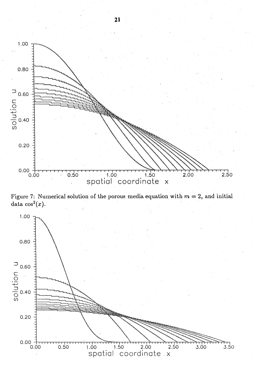
Typical obtained profiles p,re shown in Figs. 7, 8, and the evolution of the support

in Fig. 9. Note that there is a orie half factor of difference with respect to Fig. 6 of

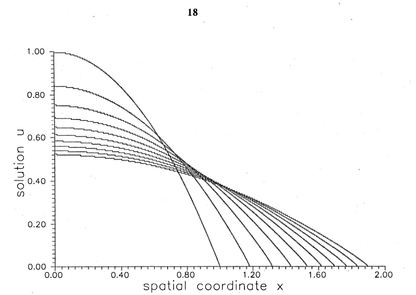
[3] . Interestingly, a close examination of Figs. 7, 8 shows the convergence, as t goes to infinity, of the solution of Ut = u2xx with the given initial data, to a Barenblatt

self,similar solution. This is a well known fact , that we show for. m = 3 in Fig. 1 0.

1 . 00

0.80

::J 0 . 60 C o +-' ::J 0 0 . 4 0 (f)

0 . 2 0

1 8

0 .00 4.����0-"",�"-.���4,,,���0-�r+��L,��,,,

0.00 0 . 4 0 0 . 8 0 1 . 2 0 .

s p a t i a l c o o rd i n a t e x

1 . 60 2 . 00

Figure 2: N umerical solution of the porous media equation with m = 2, and initial

data 1 _ x2 • .

1 . 00

0 . 80

::J 0 .. 60 �--_ C

o +-' ::J 0 0 . 4 0 (f)

0 . 2 0

0 . 0 0 --I--1",,-,-,-,rr, " '1,'0-••" ''''-'' ",,--\-.-r....-"r-o-rT'--r-ri'-.-r";-r-r--.-"1,-r"-ri'--.-"1-rl

0.00 0 . 40 . 0 . 8 0 1 . 20 1 . 60 2 . 00

s p a t i a l c o o rd i n a t e x

Figure 3 : _{Exact solution of the porous media equation with m = 2, and initial data}

1 . 0 0

0 . 8 0

:J 0.60 C o +-' :J 0 0 .40 (f)

0 . 2 0

1 9

0 . 00 4T������rM����MT��Tn���nT������n.+n�

0 . 0 0 0 . 5 0 1 . 0 0 1 . 5 0 2 . 00 2 . 50 3 . 00 3 . 5 0 4 . 0 0

s p a t i a l c o o rd i n a t e x

Figure 4: Numerical solution of the porous media equation with m = 3, and initial

data ( 1 -X2) 1/2,

1 . 00

0 . 8 0

:J 0 . 6 0 c o +-' :J 0 0 . 4 0

(f)

0 . 2 0

0 . 0 0 _{TTTlTTlCTT"nTTTTTTT+rr,TrrTTl}TTTTTTTTTTTTTn+rrrrrrrt-r 0 . 00 0 . 5 0 1 . 00 1 . 50 2 . 0 0 2 . 50 3 . 0 0

s p a t i a l c o o r d i n a t e x

3 . 5 0 4 . 0 0

Figure 5: Exact solution of th� porous media equation with m = 3 , and initial data

2 . 2 0

2 . 0 0

x (J) 1 . 80 -I-'

o C . - 1 60 -0 '

L o o U 1 . 40

o :.;::; 1 . 2 0

o 0.. (f) 1 . 0 0

20

0 . 8 0 nTTrTTTTrTTTTrTTTTrTT.,.,-rrr.,.,-rrr.,.,-rrr.,.,-rrr.,.,-rrr..,..,-rrr..,..,-rn..,..,-rn""'TT"1..,.,n 0 . 0 0 0. 1 0 0 . 2 0 0 . 30 0 . 40

t i m e t 0.50 0.60

0 . 7 0

Figure 6: Exact and numerical interface curves for the porous media equation with

m = 2.

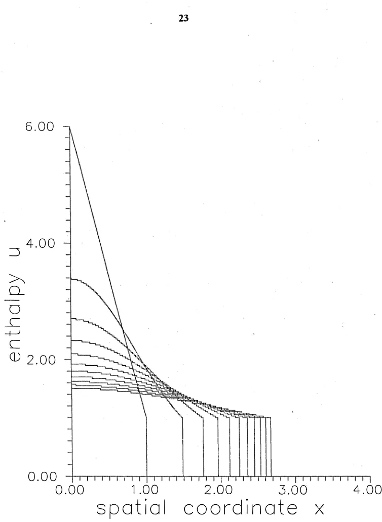
with a triangular initial profile. Its evolution is shown in Fig. 11. As a nonclassical example we include Figs. 12, 13 . One may suspect that a positive waiting time will be present, by comparison with the analogous problem for the porous media equation (Fig. 7). Numerical evidence for this waiting time is shown in Fig. 14. Practically in all cases we begin by discretising the range of the initial data, typi­ cally in 200 intervals, and taking as its approximation a linear combination of step functions . We have named Xi the abscissas of the discontinuities of the numerical initial profile. The following step is to discretise a( u) according with the assumed discretisation for Ui . · Then, we integrate in time the system of ordinary differential

1 . 00

0 .80

::J 0 . 60 C o +-' ::J 0 0. 40 (f)

0 . 2 0

21

0 .00 ������rr��.-rr�TT.,.-rr�����rr����rT",,�

0 . 0 0 . 0 . 50 1 . 00 1 . 50 s p a tia l c o o rd i n a te x

2 . 0 0 2 . 5 0

Figure 7: Numerical solution of the porous media equation with m = 2, and initial data cos2(x).

1 . 00

0 . 8 0

::J 0 . 6 0 C o +-' ::J 0 0 .40 (f)

0 . 2 0

0 . 0 0 �Trnno"no"rnTTnnTT��nrToTho,,�"��Tr�.rho,�rih�rih�n 0 . 00 0 . 50 1 . 00 1 . 50 2 . 00 2 . 50

s pa t i a l c o o rd i n a t e x

3 . 00 3 . 50

Figure 8: Numerical solution of the porous media equation with m = 2, and initial

22

1 . 8 0

;'

,/ ,/ ./

1 . 7 0

. 5*

�

X _,/

-- - C O S4

�

j

(l) _COS x ,/ ",

U "

0 ,/ ,

'+- ,

L _,/ ,

(l) ,

+-' _,/ " ,

. � 1 . 6 0 ,

/ ,

""" /' ,/

1 . 50 -h,-,--r-r-r-r--r"l-r-r-r-.,-,--,-,-,--,r-r--r-r-r-r-r-r-r-r-r-r-r-r-r..,-,-,-r-r-.,-,--,-,-r-r-r--r-r....-r-r-r1

0 . 0 0 0 . 0 5 0. 1 0 0. 1 5 0.20 0.25

" ti m e t

Figure 9: Numerical interface .curves Jor the porous media. equation with m = 2.

1 . 0 0

0 . 8 0

::J 0 . 6 0 C o +-' ::J 0 0 . 40 (f)

0 . 2 0

0.00 -!-rTTTrrr""'''TT'rrrTTTTTTrrr.,."-ri'lhTrrrTTTTTTrrr'rn",,,''''''''rrrmTTTh-r-rn*rh-fn-'rnTl 0 . 0 0 0 . 50 1 . 00 1 . 5 0 , 2 . 00 2 . 50 3 . 0 0 3 . 50 4. 0 \

s p a t i a l c o o rd i n a te x

Figure 1 0 : Numerical solution of the porous media equation with m = 3 , and initia

6 . 0 0

-=> 4 . 0 0

� u o

...c

-+---'

C

ill 2 . 0 0

0 . 0 0

0 . 0 0 1 . 0 0

s p a t i a l

23

2 . 0 0 3 . 0 0

c o o rd i n a t e

4 . 00

24

2 . 00

1 . 50

c

. Q 1 . 00 -I-'

:J o (f)

0.50

o . 0 0 . - ,--,--r-.--,-"..-r--r-r-rr-ro--,-,r-r-r-r--r-,-,-,--r-r-.-r-'-'-'-I,-r-r-r---.-r-r-r-.-r

O. 1 0

s p a ti a l c o o rd i n a te x

2 .00

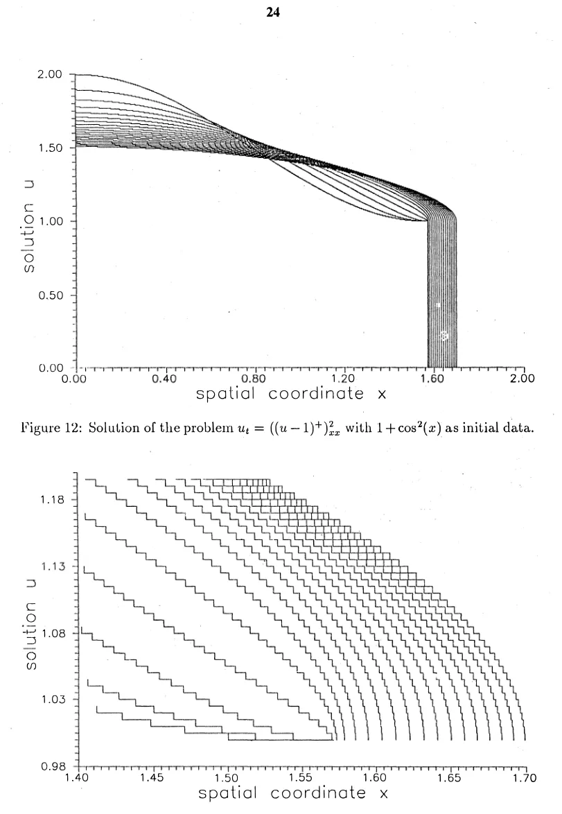
Figure 1 2 : Sol ution of the problem Ut = ((u - 1 ) + ) ;", with 1 + cos2(x} as initial d�ta.

c o

1 . 1 8

:J 1 . 08 o (f)

1 . 03

o . 9 8 --!--r-r-r-rr-'-'-r--r-J-,-,-,-,-,..,-,.--,--,-rr-r-r,..,-,.--,--,r-r-r-r-r-.--r-onrrr-r-r-rr-onrrr-,-,-,-,-,..,-,.--,--,rrT'"1

1 . 40 1 . 45 1 . 50 1 . 55 1 . 60

s pa ti a l c o o rd i n a te x

1 . 65

Figure 13: Detail of the support evolution for Fig. 12.

1 . 7 5

x 1 . 70

(j) +-' o c 1 . 6 5 "D

L o o () 1 . 6 0

o +-' o Q 1 . 5 5 (f)

25

1 . 50 --h-,-,--nrrr-<-rrT-rrrrrr-,-,--nrrnrrr-<-rrrrrr-rrn,.,..,.,.,..,.,-rrrrrr-rrn'TTT-rrrTTrrrrrrn"TTTTTTTTrrrrrrn"TTTTI 0 . 0 0 0 . 1 0 0 . 2 0 0 . 3 0 0 . 4 0 0 . 50 0 . 6 0 0 . 7 0 0 . 80 0 . 9 0

ti m e t

Figure 14: Numerical interface curve for the solution of Figs. 1 2, 13.

References

[1] D . G . Aronson. The porous medium equation, in Nonlinear Diffusion Prob­ lems. A. Fasano, M. Primicerio, Editors. Lecture Notes in Mathematics 1224.

Springer-Verlag, 1986. .

[2] J . 1 . Graveleau and P. Jamet . A finite difference approach to some degenerate nonlinear parabolic equations. SIAM J . Appl. Math. 20 ( 1 97 1 ) , 1 99-223. [3] K. Tomoeda and M . Mimura. Numerical approximations to inte:face curves for